AI glossary
Neural Network
A neural network is a machine-learning model built from layers of simple processing units, called neurons, linked by adjustable connections (weights). It learns by adjusting those weights, example after example, until its predictions on the training data are accurate, and then applies what it learned to new data. You meet them daily: large language models like ChatGPT, photo-search algorithms that find similar images, speech recognition that transcribes your voice, translation services that swap languages, and scientific tools like AlphaFold that predict protein structures. This guide explains the parts of a neural network, how it learns (with one training step worked through in real numbers), the main types, a short history from 1943 to transformers, how networks compare with the brain, where they are used and where they fail. It also includes a small experiment we ran ourselves.
The parts of a neural network
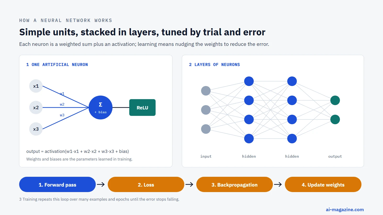
To understand how a neural network works, you need to know its anatomy. While the name suggests a biological origin, the analogy is loose. Real neurons and synapses are far more complex than their artificial namesakes (see the comparison below); the basic unit of computation is only loosely inspired by the neuron.
Neurons, weights, and biases
At the core of every neural network is the artificial neuron. It receives inputs, processes them, and passes the result to the next layer. Mathematically, each neuron computes a weighted sum of its inputs and adds a bias term. The weights determine how much influence each input has on the output, while the bias allows the model to shift the activation function left or right. This simple calculation is repeated across thousands or millions of neurons, creating a dense web of connections.
Activation functions
If neurons only performed linear calculations, the entire network would collapse into a single linear layer, no matter how many layers it had. Activation functions introduce non-linearity, allowing the network to learn complex patterns. A common choice is ReLU (Rectified Linear Unit), which outputs the input directly if it is positive, and zero otherwise. ReLU became popular after studies by Nair and Hinton (2010) and Glorot, Bordes, and Bengio (2011) showed it trained faster and more effectively than older functions like sigmoid in deep networks. Other functions, like softmax, are used in the output layer to turn raw scores into probabilities that sum to one, which is essential for classification tasks.
Layers and what “deep” means
Neural networks are organized into layers. The input layer receives the raw data, such as pixel values or word embeddings. Hidden layers sit between the input and output, transforming the data step by step. The output layer produces the final prediction, like a category label or a continuous value. When a network has many hidden layers, it is called a “deep” neural network, and the field is referred to as deep learning. The depth allows the network to learn hierarchical features: early layers might detect edges in an image, while deeper layers recognize complex objects like faces or cars. This layered structure is what enables neural networks to approximate highly complex functions, a capability formally described by the universal approximation theorem.
How a neural network learns
Training a neural network is the process of teaching it to make accurate predictions. It involves feeding data through the network, measuring the error, and adjusting the weights to minimize that error. This cycle repeats many times until the network performs well on unseen data.
Forward pass and loss
Training begins with a forward pass. Data enters the input layer and flows through the hidden layers, with each neuron applying its weights, biases, and activation functions. The final output is compared to the known correct answer using a loss function. For classification tasks, the most common loss function is cross-entropy, which measures the difference between the predicted probability distribution and the true labels. The goal of training is to minimize this loss value.
Backpropagation and optimization
Once the loss is calculated, the network needs to figure out which weights contributed to the error. Backpropagation, or backprop, does this by applying the chain rule of calculus to compute the gradient of the loss with respect to each weight. It essentially traces the error backward from the output layer to the input layer, assigning responsibility for the error to each connection. An optimizer, such as stochastic gradient descent or Adam, uses these gradients to update the weights. Adam, introduced by Kingma and Ba in 2014, is widely used because it adapts the learning rate for each parameter, often leading to faster and more stable convergence. Techniques like batch normalization (Ioffe & Szegedy, 2015) also help by stabilizing the learning process, allowing networks to reach the same accuracy with significantly fewer training steps.
Epochs, overfitting, and hyperparameters
Training happens in epochs, where each epoch is one full pass through the entire dataset. However, training too long can lead to overfitting, where the network memorizes the training data but fails to generalize to new examples. To prevent this, developers use techniques like dropout, which randomly disables neurons during training (Srivastava et al., JMLR 2014), forcing the network to learn redundant representations. Another strategy is using a validation set to monitor performance on unseen data and stopping training when errors start to rise. It is important to distinguish between parameters and hyperparameters. Parameters are the weights and biases learned during training. Hyperparameters, such as the number of layers, learning rate, and batch size, are set by the developer before training begins and control how the learning process unfolds.
The universal approximation theorem
A foundational concept in neural networks is the universal approximation theorem. Proven by Cybenko (1989) and Hornik (1991), it states that a neural network with just one hidden layer and enough units can approximate any continuous function to any desired accuracy. This means that, theoretically, a network could learn any pattern given enough capacity. However, the theorem says such a network exists; it does not guarantee that training will find it, nor does it ensure the network will be efficient or practical. In practice, deep networks with many layers are often preferred because they can learn complex functions with fewer total parameters than a single wide layer.
A worked example: one training step with real numbers
Here is a tiny network doing one forward pass and one weight update, with every number shown. It has two inputs, two hidden neurons with ReLU, and one output neuron with a sigmoid that turns the score into a probability. The training example is the input (1, 0) with the correct answer 1.
Forward pass
| Step | Calculation | Result |
|---|---|---|
| Hidden neuron 1 | 1 × 0.5 + 0 × 0.3 + bias 0.0 = 0.5 → ReLU | 0.5 |
| Hidden neuron 2 | 1 × (−0.4) + 0 × 0.8 + bias 0.1 = −0.3 → ReLU | 0 |
| Output score | 0.5 × 0.7 + 0 × (−0.2) + bias 0.05 | 0.40 |
| Probability | sigmoid(0.40) | 0.599 |
| Loss | cross-entropy = −ln(0.599) | 0.513 |
The network is 59.9% sure the answer is 1. It should be 100% sure, so the loss is 0.513.
Backward pass and update
For a sigmoid output with cross-entropy loss, the gradient of the loss with respect to the output score is simply prediction − target = 0.599 − 1 = −0.401. The gradient for the weight from hidden neuron 1 to the output is that number times the neuron’s output: −0.401 × 0.5 = −0.201. With a learning rate of 0.5, gradient descent changes the weight by −0.5 × (−0.201), from 0.70 to 0.80.
Run the forward pass again and the probability rises to 0.611 and the loss falls to 0.493. Notice two things. Hidden neuron 2 output 0, so its outgoing weight got no gradient at all in this step: ReLU units that are switched off do not learn from that example. And the change is small; real training repeats this millions or billions of times, across every weight at once, which is exactly what backpropagation computes efficiently.
Types of neural networks
Neural networks are not one-size-fits-all. Different architectures are designed to handle specific types of data and problems. Below are the most common types, their origins, and their primary use cases.
Feedforward networks (MLPs)
The simplest type is the feedforward network, also known as a multilayer perceptron (MLP). Data flows in one direction from input to output without looping back. These networks are best suited for tabular data and simple classification tasks. While they form the basis of more complex architectures, they struggle with data that has spatial or temporal structure, like images or text sequences.
Convolutional neural networks (CNNs)
Convolutional neural networks, or CNNs, were pioneered by Yann LeCun, who in 1989 trained one to read handwritten zip codes (the LeNet paper followed in 1998). CNNs are designed to process grid-like data, such as images and video. They use convolutional layers that apply filters to detect local patterns like edges, textures, and shapes. This architecture drastically reduces the number of parameters compared to fully connected networks, making it highly efficient for visual tasks. CNNs dominated computer vision for years, leading to breakthroughs like AlexNet in 2012 and ResNet in 2015 (image recognition algorithms explained).
Recurrent neural networks (RNNs, LSTM, GRU)
Recurrent neural networks, or RNNs, are designed for sequential data, such as time series or text. They have internal memory that allows information to persist as the network processes a sequence. However, standard RNNs struggle with long-range dependencies. To solve this, Hochreiter and Schmidhuber introduced Long Short-Term Memory (LSTM) networks in 1997. Later, Cho et al. introduced the Gated Recurrent Unit (GRU) in 2014 as a simpler, faster alternative. While powerful, RNNs and their variants have largely been replaced by transformers for language tasks due to efficiency and performance gains.
Autoencoders
Autoencoders are neural networks trained to reconstruct their input. They consist of an encoder that compresses the input into a lower-dimensional representation and a decoder that reconstructs it. Hinton and Salakhutdinov (Science 2006) demonstrated how to train deep autoencoders effectively. They are commonly used for anomaly detection, dimensionality reduction, and data compression. By learning the underlying structure of the data, autoencoders can identify outliers or generate new data samples that resemble the training set.
Generative Adversarial Networks (GANs)
Introduced by Goodfellow et al. in 2014, GANs consist of two networks: a generator and a discriminator. The generator creates fake data, while the discriminator tries to distinguish between real and fake data. They compete in a zero-sum game, pushing both to improve. GANs are renowned for their ability to generate highly realistic images, videos, and audio. They have become a cornerstone of generative AI, enabling applications like style transfer, image super-resolution, and synthetic data generation.
Transformers
The transformer architecture, introduced in 2017 in the paper “Attention Is All You Need,” revolutionized machine learning. Unlike RNNs, transformers process all tokens in a sequence simultaneously using attention mechanisms, which allow the model to weigh the importance of different parts of the input. This architecture dispenses with recurrence and convolutions entirely. Transformers are the foundation of modern large language models (LLMs) like GPT, Claude, and Llama. They excel at language tasks, code generation, and increasingly at image and audio processing.
Graph neural networks (GNNs)
Graph neural networks, or GNNs, are designed to work with graph-structured data, where entities are nodes and relationships are edges. Scarselli et al. (2009) laid the groundwork, and Kipf and Welling (2017) advanced the field with graph convolutional networks. GNNs are used in social network analysis, recommendation systems, molecular modeling, and traffic prediction. They capture complex relationships and dependencies that traditional neural networks might miss.
Diffusion models
Diffusion models, popularized by Ho, Jain, and Abbeel in 2020 with the Denoising Diffusion Probabilistic Model (DDPM), generate data by gradually adding noise to an image and then learning to reverse the process. They have become a leading approach for high-quality image and video generation, competing with and often surpassing GANs in fidelity. Image generators such as Stable Diffusion are built on this approach.
Spiking neural networks
Spiking neural networks (SNNs) are inspired more closely by biological neurons. They communicate via discrete electrical spikes rather than continuous values. Maass (1997) described them as a “third generation” of neural networks. On neuromorphic hardware they can be very energy-efficient. They are still largely in the research phase but hold promise for low-power AI applications and real-time sensory processing.
| Type | Introduced | Best for | Example |
|---|---|---|---|
| Feedforward / MLP | 1958 perceptron; multilayer training 1986 | Tabular data, simple classification | Digit classifier below |
| CNN | 1989 (LeCun) | Images, video | AlexNet, ResNet |
| RNN / LSTM / GRU | 1997 (LSTM), 2014 (GRU) | Sequences, time series | Early speech recognition |
| Autoencoder | Deep autoencoders 2006 (Hinton, Salakhutdinov) | Anomaly detection, compression | Data denoising |
| GAN | 2014 (Goodfellow) | Image generation | StyleGAN |
| Transformer | 2017 | Language, code, multimodal | GPT-4, Llama 3 |
| GNN | 2009 (Scarselli et al.) | Graphs, networks | Molecular property prediction |
| Diffusion | 2020 (DDPM) | High-fidelity image/video | Stable Diffusion |
| Spiking | 1997 (Maass) | Neuromorphic chips, low power | Event-based vision |
We trained one: a neural network vs a simpler model
To show what neural networks do well and where they are unnecessary, we ran two small experiments with scikit-learn 1.9.1 on a laptop on 15 October 2026.
Experiment 1: XOR. XOR outputs 1 when exactly one of two inputs is 1. It is the problem Minsky and Papert used in 1969 to show the limits of single-layer perceptrons. A single perceptron got 2 of the 4 cases right, no better than guessing, because no straight line separates the classes. A network with one hidden layer of just two neurons can solve it, but in our runs it found the solution in only 2 of 5 random starting points; in the others it got stuck in a poor local minimum. That is a small-scale picture of why initialization and optimizers matter.

Experiment 2: handwritten digits. We used scikit-learn’s digits dataset: 1,797 images of handwritten digits, each 8 × 8 pixels (64 inputs), split into 1,347 training and 450 test images.
| Model | Parameters | Test accuracy |
|---|---|---|
| Logistic regression (no hidden layer) | 650 | 96.9% |
| Neural network, 1 hidden layer of 4 neurons | 310 | 87.3% |
| Neural network, 1 hidden layer of 16 neurons | 1,210 | 96.0% |
| Neural network, 1 hidden layer of 64 neurons | 4,810 | 97.3% |
| Neural network, 2 hidden layers of 64 neurons | 8,970 | 97.6% |
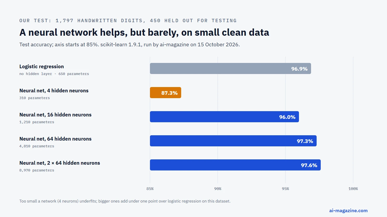
A network that is too small (4 hidden neurons) underfits and does worse than plain logistic regression. Bigger networks reach 100% on the training images and 97–98% on the test images, but on a dataset this small and clean they beat the simple model by less than one percentage point. Neural networks earn their cost on large, messy data such as photos, audio and text, where simpler models fall far behind.
from sklearn.datasets import load_digits
from sklearn.model_selection import train_test_split
from sklearn.neural_network import MLPClassifier
from sklearn.preprocessing import StandardScaler
from sklearn.pipeline import make_pipeline

X, y = load_digits(return_X_y=True)
X_tr, X_te, y_tr, y_te = train_test_split(X, y, test_size=0.25, random_state=0, stratify=y)

model = make_pipeline(StandardScaler(),
                      MLPClassifier(hidden_layer_sizes=(64, 64), max_iter=600, random_state=0))
model.fit(X_tr, y_tr)
print(f"test accuracy: {model.score(X_te, y_te):.3f}")  # 0.976 in our run
A short history of neural networks
The story of the neural network begins in 1943, when Warren McCulloch and Walter Pitts published “A logical calculus of the ideas immanent in nervous activity.” This paper presented the first mathematical model of a neuron, showing that simple units connected in specific patterns could perform logical operations. It was a theoretical foundation, not yet a practical tool. A decade later, in 1958, Frank Rosenblatt introduced the perceptron, a single-layer learning machine. The U.S. Office of Naval Research demonstrated it on an IBM 704 computer, generating significant excitement. However, the hype was short-lived.
In 1969, Marvin Minsky and Seymour Papert published “Perceptrons,” a critical analysis that highlighted the limitations of single-layer networks. They demonstrated that these networks could not solve simple problems like XOR (exclusive OR) without additional layers. This mathematical proof, combined with hardware limitations, caused interest to drop. Neural networks entered a period often called the “AI winter,” where funding dried up and research slowed for nearly two decades.
The field began to revive in the 1970s and 1980s as researchers found ways to train deeper networks. In 1974, Paul Werbos proposed applying backpropagation, a method to calculate how much each weight contributed to the error, to neural networks in his Harvard PhD thesis. By 1982, John Hopfield introduced networks that could serve as content-addressable memory systems. The real breakthrough came in 1986, when David Rumelhart, Geoffrey Hinton, and Ronald Williams published “Learning representations by back-propagating errors.” This paper made training multi-layer networks practical, allowing networks to learn complex patterns by adjusting weights through the chain rule.
The 1990s saw specialized architectures emerge. Yann LeCun applied backpropagation to convolutional networks to read handwritten zip codes, publishing the LeNet paper in 1998. Around the same time, Sepp Hochreiter and Jürgen Schmidhuber introduced long short-term memory (LSTM) networks in 1997 to handle sequential data. Despite these advances, computing power remained a bottleneck. It wasn’t until 2006 that Hinton and colleagues demonstrated how to train deep networks layer by layer using “deep belief nets,” effectively restarting the deep learning revolution.
The 2010s marked the era of massive scale and performance. In 2012, AlexNet won the ImageNet competition with a top-5 error rate of 15.3%, dramatically outperforming the runner-up at 26.2%. It showed that deep convolutional networks trained on GPUs could beat hand-engineered computer vision by a wide margin. The field continued to evolve with generative adversarial networks (GANs) in 2014 and ResNet in 2015, which achieved 3.57% error on ImageNet with up to 152 layers.
A paradigm shift occurred in 2017 with the introduction of the transformer architecture. The paper “Attention Is All You Need” described a model based solely on attention mechanisms, dispensing with recurrence and convolutions entirely. This architecture became the foundation for today’s large language models. The contributions of the field’s pioneers were recognized with the 2018 ACM Turing Award, announced in March 2019, given to Yoshua Bengio, Geoffrey Hinton, and Yann LeCun. In 2024, the Nobel Prize in Physics was awarded to John Hopfield and Geoffrey Hinton for foundational discoveries enabling machine learning with artificial neural networks.
| Year | Milestone | Who |
|---|---|---|
| 1943 | First mathematical model of a neuron | Warren McCulloch, Walter Pitts |
| 1958 | Perceptron demonstration | Frank Rosenblatt |
| 1969 | Limits of single-layer perceptrons | Marvin Minsky, Seymour Papert |
| 1974 | Backpropagation proposal | Paul Werbos |
| 1982 | Hopfield networks | John Hopfield |
| 1986 | Practical backpropagation for multi-layer networks | David Rumelhart, Geoffrey Hinton, Ronald Williams |
| 1989 | Convolutional network for zip codes | Yann LeCun |
| 1997 | LSTM | Sepp Hochreiter, Jürgen Schmidhuber |
| 2006 | Deep belief nets | Geoffrey Hinton et al. |
| 2012 | AlexNet wins ImageNet | Alex Krizhevsky et al. |
| 2015 | ResNet | Kaiming He et al. |
| 2017 | Transformer architecture | Ashish Vaswani et al. |
| 2018 | ACM Turing Award (announced 2019) | Yoshua Bengio, Geoffrey Hinton, Yann LeCun |
| 2024 | Nobel Prize in Physics | John Hopfield, Geoffrey Hinton |
Neural network vs the human brain
When people hear “neural network,” they often imagine a digital copy of the human brain. The analogy is useful for beginners but technically loose. Both systems use interconnected units to process information, but their structures and scales differ significantly.
The human brain contains approximately 86 billion neurons, according to research by Azevedo et al. in 2009. This number is lower than the commonly cited 100 billion. These neurons are connected by roughly 150 trillion synapses in the neocortex, as reported by Pakkenberg et al. in 2003. A synapse is a complex biological structure involving chemical and electrical signaling, not just a simple weight.
In contrast, a neural network parameter is a single number representing a connection strength. The scale comparison looks similar on the surface but misses the biological complexity. For instance, AlexNet in 2012 had 60 million parameters. By 2020, GPT-3 scaled to 175 billion parameters. The 2024 Llama 3.1 model reached 405 billion parameters in a dense configuration. Even larger models like DeepSeek-V3, released in December 2024, have 671 billion total parameters, with only 37 billion active per token in a mixture-of-experts architecture.
On raw counts, the largest models now have more parameters than the brain has neurons, but far fewer than the neocortex has synapses, and the comparison is misleading either way. Biological neurons do more than pass weighted sums; they integrate signals over time, use diverse neurotransmitters, and adapt structurally. Neural networks simplify this into mathematical functions like ReLU or sigmoid. While the brain is energy-efficient and learns continuously, neural networks require massive datasets and computational power. The comparison holds for the concept of connected units, but the implementation details are fundamentally different.
| System | Count |
|---|---|
| Human brain neurons | ~86 billion |
| Human brain synapses (neocortex) | ~150 trillion |
| AlexNet (2012) parameters | 60 million |
| GPT-3 (2020) parameters | 175 billion |
| Llama 3.1 (2024) parameters | 405 billion |
| DeepSeek-V3 (2024) total parameters | 671 billion |
Where neural networks are used
Neural networks have moved from research labs into everyday applications. Their ability to recognize patterns in unstructured data has transformed several industries.
In language processing, large language models like GPT, Claude, Gemini, and Llama are transformer-based neural networks. They generate text, code, and summaries by predicting the next token in a sequence. These models handle tasks ranging from customer service chatbots to complex reasoning, though their internal workings remain largely opaque.
Image recognition is another major domain. Convolutional neural networks (CNNs) excel at identifying objects, faces, and scenes. ResNet achieved a top-5 error rate of 3.57% on the ImageNet dataset in 2015. This technology powers facial recognition, medical imaging analysis, and autonomous vehicle vision systems.
Speech recognition has also seen dramatic improvements. In 2016, Microsoft reported a system that matched professional human transcribers on the Switchboard benchmark. The human error rate was 5.9%, while the system achieved 5.8% in a later version. This parity marked a significant milestone in natural language processing.
Machine translation relies heavily on neural networks. Google’s Neural Machine Translation (GNMT) system, introduced in 2016, used deep LSTM networks. It reduced translation errors by about 60% compared to its previous phrase-based system, based on human side-by-side evaluations of isolated simple sentences. This improvement made real-time translation more accurate and fluent.
In biology, AlphaFold made headlines in 2021 by predicting protein structures with high accuracy. Its open database now contains over 200 million predicted structures, accelerating drug discovery and biological research. This application demonstrates how neural networks can solve complex scientific problems that were previously intractable.
Recommendation systems, used by streaming services and e-commerce platforms, also rely on neural networks to predict user preferences. These models analyze past behavior to suggest movies, products, or content, keeping users engaged.
Other applications include anomaly detection in manufacturing, fraud detection in finance, and generative AI for creating images and audio. The versatility of neural networks continues to expand as models grow larger and more efficient.
Limitations of neural networks
Despite their success, neural networks have significant limitations that prevent them from being universal solutions.
Adversarial examples highlight a vulnerability where tiny, imperceptible changes to input data can cause misclassification. Szegedy et al. demonstrated this in 2013. Goodfellow et al. in 2014 showed a striking example: an image of a panda classified as “panda” with 57.7% confidence became classified as a “gibbon” with 99.3% confidence after an invisible perturbation. This suggests that networks may rely on superficial patterns rather than deep understanding.
Opacity is another challenge. Neural networks are often described as black boxes because it is difficult to explain why they make specific decisions. Anthropic’s 2024 research on “Scaling Monosemanticity” extracted up to about 34 million interpretable “features” from its Claude 3 Sonnet model. While this provides some insight, most network behavior remains unexplained, making trust difficult in critical applications like healthcare or law.
Catastrophic forgetting occurs when a network learns a new task and overwrites knowledge from previous tasks. McCloskey and Cohen identified this in 1989. This is a major hurdle for continuous learning systems that need to adapt without retraining from scratch.
The “double descent” phenomenon, described by Belkin et al. in 2018 and Nakkiran et al. in 2019, shows that test error can fall, rise, and fall again as models grow larger. This complicates the textbook bias-variance picture, in which larger models simply overfit more. It implies that simply adding parameters does not always lead to better generalization in the expected way.
Data and energy demands are substantial. Large models require massive datasets; DeepSeek-V3 was trained on 14.8 trillion tokens. Training and running these models consume significant electricity. Data centers used about 415 TWh of electricity in 2024, about 1.5% of the world’s electricity consumption, according to the IEA. While not all of this is for AI, the trend is upward. Epoch AI (2026) notes that training compute for frontier language models has grown about 5x per year since 2020.
Finally, neural networks are not always the best choice. On small tabular datasets, simpler models like decision trees or logistic regression often match or beat neural networks, as our experiment above shows. They require less data and are easier to interpret. Using a complex neural network for a simple problem can be inefficient and unnecessary.
How to start building one
Building a neural network is accessible thanks to modern tools. You do not need a PhD to start experimenting.
For beginners, TensorFlow Playground is an excellent starting point. This interactive tool allows you to train a small network in the browser. It visualizes weights, activations, and loss in real-time, helping you understand how data flows through layers. It is ideal for grasping the basics of forward pass and backpropagation without writing code.
Once you are comfortable with the concepts, move to Python frameworks. PyTorch and TensorFlow/Keras are the industry standards; our framework comparison helps you choose. PyTorch is known for its dynamic computation graph and intuitive syntax, making it popular in research and increasingly in production. TensorFlow/Keras offers a high-level API that simplifies model creation and deployment. Both have extensive documentation and community support.
A suggested learning order is:
- Understand the basics: Use TensorFlow Playground to see how neurons and layers work.
- Learn Python: Ensure you are comfortable with Python, as it is the primary language for AI.
- Start with Keras: Use Keras’ high-level API to build your first model. It abstracts away many complexities, letting you focus on architecture and data.
- Explore PyTorch: As you advance, learn PyTorch for more control and flexibility, especially for custom architectures.
- Experiment: Train models on small datasets like MNIST or Iris to see how changes in layers and hyperparameters affect performance.
Remember that training takes time and computational resources. Start small, monitor your loss curves, and iterate. The key is hands-on practice.
FAQ
What is a neural network in simple terms?
A neural network is a machine-learning model inspired by the brain, made of layers of simple units called neurons. These neurons are connected by weighted links that adjust during training. The network processes input data through these layers to produce a prediction or classification. It learns by adjusting weights to minimize errors.
How does a neural network learn?
A neural network learns through a process called backpropagation. It makes a prediction, calculates the error using a loss function, and then adjusts its weights to reduce that error. This process repeats over many examples and epochs. Optimizers like Adam or gradient descent guide the weight updates. The goal is to find weights that generalize well to new data.
What is the difference between a neural network and deep learning?
A neural network is a single model with one or more hidden layers. Deep learning refers specifically to neural networks with many hidden layers, often called “deep” networks. The term “deep” highlights the complexity and depth of the architecture. All deep learning models are neural networks, but not all neural networks are considered deep learning.
What are the main types of neural networks?
Common types include feedforward networks (MLPs) for tabular data, convolutional networks (CNNs) for images, and recurrent networks (RNNs) for sequences. Transformers are now dominant for language. Other types include autoencoders for compression, GANs for generation, and graph neural networks for structured data. Each type is optimized for specific data structures.
Is a neural network the same as AI?
No, a neural network is a specific technique within the broader field of artificial intelligence. AI includes many methods like search algorithms, rule-based systems, and symbolic reasoning. Neural networks are a subset of machine learning, which is a subset of AI. They excel at pattern recognition but do not encompass all AI capabilities.
How many layers does a neural network need?
The number of layers depends on the task. Simple problems may require only one hidden layer, as shown by the universal approximation theorem. Complex tasks like image or language processing often need many layers, forming deep networks. There is no fixed number; more layers increase capacity but also computational cost and the risk of overfitting.
Are neural networks like the human brain?
The analogy is loose. Both use interconnected units to process information. However, the brain has billions of neurons and trillions of synapses, with complex biological mechanisms. Neural networks use mathematical functions and parameters. The brain is energy-efficient and continuously learning, while networks require massive data and compute. They share a conceptual similarity but differ in implementation and scale.