How Transformer Attention Actually Works
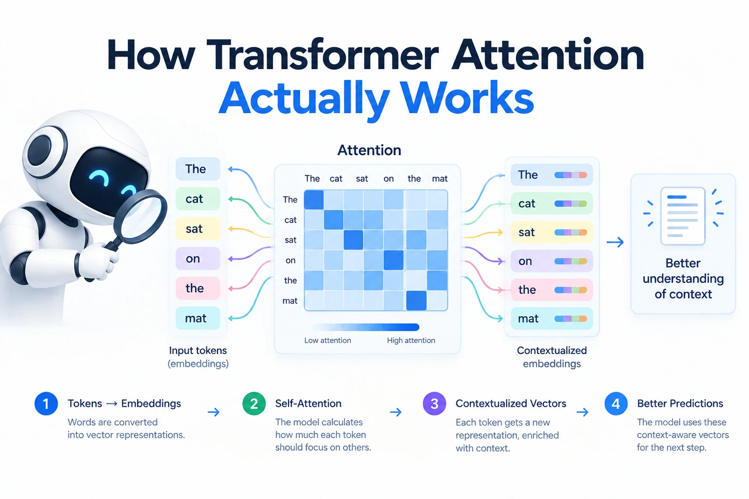
Attention, the mechanism behind every model discussed elsewhere on this site, is one formula: Attention(Q, K, V) = softmax(QKᵀ/√d_k)V. That’s it — three matrices, one dot product, one softmax. The diagram on this site’s own homepage (query tokens, key tokens, and the weighted lines connecting them) is a direct visualization of this exact computation, and this guide explains precisely what it’s doing, with real code and the two papers that actually invented it.
Before attention: a fixed-length bottleneck
Attention wasn’t introduced by the Transformer — it’s three years older, and it solved a narrower problem first. In September 2014, Dzmitry Bahdanau, Kyunghyun Cho, and Yoshua Bengio published “Neural Machine Translation by Jointly Learning to Align and Translate.” At the time, machine translation used an encoder-decoder RNN: the encoder compressed an entire source sentence into one fixed-length vector, and the decoder generated a translation from that single vector alone. Bahdanau’s team identified the obvious weakness — a long sentence compressed into one vector loses information — and proposed letting the decoder “(soft-)search for parts of a source sentence that are relevant,” rather than relying on one fixed summary. That soft-search is the first attention mechanism: a learned weighting over the source, computed fresh for every output word.
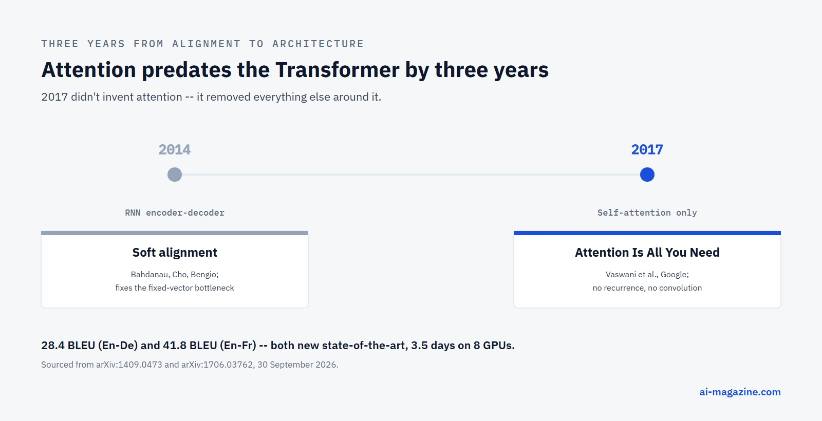
Three years later, in June 2017, eight researchers at Google — Ashish Vaswani, Noam Shazeer, Niki Parmar, Jakob Uszkoreit, Llion Jones, Aidan Gomez, Lukasz Kaiser, and Illia Polosukhin — published “Attention Is All You Need.” Their claim, right in the abstract: you don’t need the recurrent or convolutional layers at all. A network built “based solely on attention mechanisms” — no recurrence, no convolutions — beat the existing best translation models while training faster. That architecture is the Transformer, and it’s the ancestor of every model discussed in this site’s Keras, PyTorch, and TensorFlow guides.
The formula, one piece at a time
Every position in a self-attention layer is projected into three vectors: a query (what this position is looking for), a key (what this position offers to others), and a value (the actual content it contributes if attended to). The full computation, exactly as written in the original paper:
Attention(Q, K, V) = softmax(QKᵀ / √d_k) VQKᵀ computes a raw relevance score between every query and every key at once — a matrix multiplication, not a loop. Dividing by √d_k (the square root of the key dimension) keeps those scores in a stable numeric range regardless of how large the vectors are — the next section shows exactly why that matters. softmax turns each row of scores into weights that sum to 1. Multiplying by V produces, for every position, a weighted blend of every value in the sequence — weighted exactly by how relevant each one was judged to be.
Here it is as actual, runnable NumPy — no framework, no hidden magic:
import numpy as np

def softmax(x, axis=-1):
    x = x - np.max(x, axis=axis, keepdims=True)
    e = np.exp(x)
    return e / np.sum(e, axis=axis, keepdims=True)

def attention(Q, K, V):
    d_k = Q.shape[-1]
    scores = Q @ K.T / np.sqrt(d_k)
    weights = softmax(scores, axis=-1)
    return weights @ V, weights
Run against four random 8-dimensional positions (np.random.seed(0)), this is the actual output — not illustrative numbers, the real result of running the code above:
>>> Q = np.random.randn(4, 8)   # seeded, seed=0
>>> K = np.random.randn(4, 8)
>>> V = np.random.randn(4, 8)
>>> out, weights = attention(Q, K, V)
>>> weights
[[0.301 0.301 0.191 0.207]
 [0.258 0.382 0.244 0.116]
 [0.09  0.076 0.122 0.712]
 [0.82  0.086 0.023 0.072]]
>>> weights.sum(axis=1)
[1. 1. 1. 1.]
Every row sums to exactly 1 — that’s softmax doing its job, turning arbitrary scores into a genuine probability distribution over “how much attention to pay to each position.” Row 3 ([0.09, 0.076, 0.122, 0.712]) means: to compute that position’s output, blend in 71.2% of position 4’s value, and much smaller slices of the rest.
Why divide by √d_k specifically
This isn’t an arbitrary constant. The paper’s own reasoning: for query and key vectors with unit-variance components, a dot product between them is a sum of d_k independent terms — and the variance of a sum of independent terms grows with the number of terms. That means raw dot products get larger in magnitude purely because the vectors are longer, not because the match is any better. Here’s that growth, measured directly rather than asserted:
>>> for d_k in [8, 64, 512]:
...     Q, K = np.random.randn(2000, d_k), np.random.randn(2000, d_k)
...     dots = (Q * K).sum(axis=1)
...     print(d_k, dots.std(), (dots / np.sqrt(d_k)).std())
8    2.78   0.98
64   7.98   1.00
512  22.93  1.01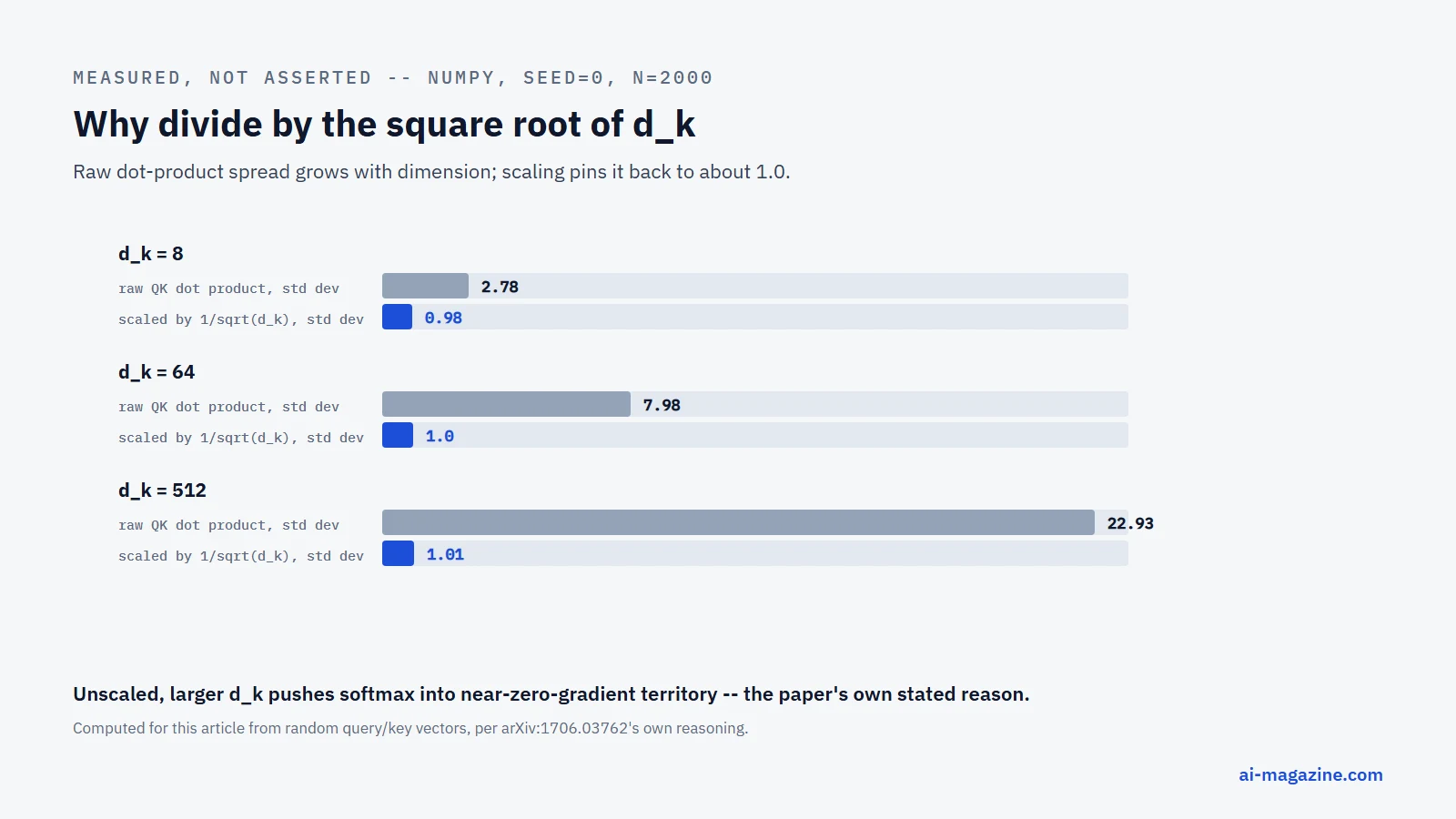
The raw standard deviation climbs roughly with √d_k (2.78 → 7.98 → 22.93, tracking √8 ≈ 2.83, √64 = 8, √512 ≈ 22.6 almost exactly) — and dividing by √d_k pins it back to right around 1.0 no matter how large the vectors get. The paper’s own explanation for why this matters: without it, “the dot products grow large in magnitude, pushing the softmax function into regions where it has extremely small gradients” — meaning the network would struggle to learn anything from those comparisons at all. The √d_k isn’t a tuning knob; it’s a fix for a specific, provable numerical problem.
Multi-head attention: several of these, in parallel
A single attention computation forces the model into one notion of “relevant.” The paper’s fix, used in every modern transformer: run several attention computations side by side, each with its own learned projections, then combine them:
MultiHead(Q, K, V) = Concat(head₁, ..., head_h) W^O
where head_i = Attention(QW_i^Q, KW_i^K, VW_i^V)
The original Transformer used h = 8 heads, with each head’s query/key/value dimension set to d_k = d_v = d_model / h = 64 (for their 512-dimensional model). Splitting one 512-dimensional attention into eight 64-dimensional ones costs about the same to compute — but each head is now free to specialize. In practice, different heads reliably learn different relationships: some track nearby words for local grammar, others connect a pronoun to a noun many words earlier.
Why this replaced recurrence: the complexity argument
The paper justifies dropping recurrence entirely with a direct complexity comparison, not just an empirical result:
| Layer type | Complexity per layer | Sequential operations | Max path length |
|---|---|---|---|
| Self-attention | O(n² · d) | O(1) | O(1) |
| Recurrent | O(n · d²) | O(n) | O(n) |
| Convolutional | O(k · n · d²) | O(1) | O(log_k(n)) |
Two things matter here. First, sequential operations: a recurrent layer needs n sequential steps to process a sequence of length n — step 50 can’t start before step 49 finishes. Self-attention needs exactly one step, since every position attends to every other position in a single matrix multiplication — which is why it parallelizes on GPUs so well. Second, maximum path length: in a recurrent network, information from position 1 has to pass through every intermediate position to reach position 500, weakening the signal along the way. In self-attention, that path length is always 1 — any two positions connect directly, regardless of distance.
The trade-off is honest, not hidden: self-attention’s O(n²) term means cost grows quadratically with sequence length, which is exactly the reason long-context handling and techniques like the KV cache matter so much in practice — the paper itself flags this and notes attention “could be restricted to a neighborhood” for very long sequences, an idea later long-context research builds on directly.
Results: what this bought in 2017
The Transformer wasn’t a theoretical curiosity — it set new state-of-the-art scores immediately. On the WMT 2014 English-to-German translation task, it scored 28.4 BLEU, more than 2 BLEU above the best previous result — including ensembles of multiple models. On English-to-French, it reached 41.8 BLEU, a new single-model state of the art, after training for 3.5 days on eight GPUs — a small fraction of the training cost of the previous best published models.
Frequently asked questions
What is the attention mechanism in one sentence?
A way for a model to compute, for every position in a sequence, a weighted blend of every other position’s information — with the weights learned from how relevant each comparison is, via softmax(QKᵀ/√d_k)V.
Who invented attention, and when?
Dzmitry Bahdanau, Kyunghyun Cho, and Yoshua Bengio introduced the first attention mechanism in September 2014, for RNN-based machine translation. The self-attention-only Transformer architecture came later, from Ashish Vaswani and seven colleagues at Google, in June 2017’s “Attention Is All You Need.”
Why is the dot product scaled by the square root of d_k?
Because raw dot products between vectors grow larger in magnitude as the vector dimension grows, purely from summing more terms — not because the match is better. Left unscaled, this pushes softmax into a region with extremely small gradients, making the network hard to train. Dividing by √d_k keeps the scale roughly constant regardless of dimension.
What is multi-head attention?
Running several independent attention computations in parallel, each with its own learned query/key/value projections, then concatenating the results. It lets different heads specialize in different kinds of relationships — for example, local grammar versus long-range reference — rather than forcing one attention pattern to capture everything.
Is self-attention always faster than recurrent networks?
Only when sequence length is smaller than the model’s representation dimension, which is the paper’s own stated condition and true for most sentence-level text. Self-attention’s cost grows quadratically with sequence length (O(n²)), so for very long sequences the comparison isn’t automatic — this is exactly the practical problem long-context techniques and KV caching address.
Related
- Uncensored AI Models: What They Are and How They’re Made, a technique that operates directly on residual-stream activations
- Keras: What It Is, How It Works, and How to Use It in 2026, PyTorch, and TensorFlow, the frameworks that implement this
- Prompt Caching: How It Works and What It Actually Saves, which relies directly on how attention’s keys and values are computed
- Attention mechanism and transformer in the glossary
- KV cache and tokens in the glossary