Genetic Algorithms Explained: How They Work, Examples and Python Code (2026)
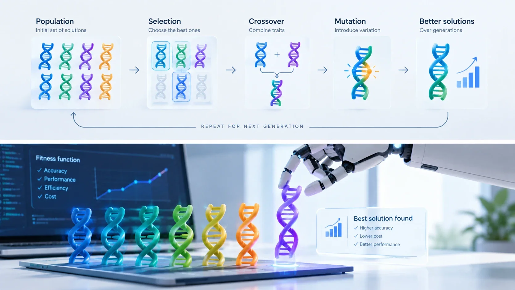
A genetic algorithm (GA) is a search method that evolves a population of candidate solutions using selection, crossover and mutation. It treats optimization like natural evolution, where the fittest individuals survive to pass their traits to the next generation. You will find these algorithms solving complex routing problems, designing antennas, and even discovering new mathematical formulas. This guide explains how a GA works step by step, gives a complete Python example you can run, walks through the history from Alan Turing to Google DeepMind’s AlphaEvolve, shows real applications, explains when a GA is the wrong tool, compares libraries, and reports a test we ran ourselves on two classic problems.
What is a genetic algorithm?
At its core, a genetic algorithm (GA) is an iterative optimization technique inspired by biological evolution. It starts with a population of random solutions, evaluates their fitness, and then applies genetic operators to create a new generation. Over time, the population converges toward better solutions. The process mimics natural selection: individuals with higher fitness scores are more likely to be selected as parents, and their genetic material is combined and mutated to produce offspring.
The biological analogy is useful but imperfect. In nature, evolution has no specific goal; it simply favors survival in a given environment. In a GA, the “environment” is defined by the fitness function you design. If the fitness function is poorly constructed, the algorithm might converge quickly to a solution that is technically “fit” but not useful for your actual problem. And unlike nature, a GA runs for a few hundred or thousand generations on a computer, with a designer choosing the encoding, the operators and when to stop.
Genetic algorithms are part of a broader family called evolutionary algorithms (EAs). Other members include evolution strategies (ES), which focus on continuous parameter optimization; evolutionary programming (EP), which often optimizes finite state machines; and genetic programming (GP), which evolves entire computer programs or tree structures rather than fixed-length strings. While these methods share the same evolutionary philosophy, they differ in how they represent solutions and which operators they prioritize. Holland’s work laid the foundation for GAs, while Rechenberg and Schwefel advanced ES, and Koza pioneered GP. Understanding where GAs fit in this family helps you choose the right tool for the job. For instance, if you are optimizing neural network weights, you might lean toward evolution strategies. If you are evolving code, genetic programming is more appropriate.
How a genetic algorithm works

To understand how genetic algorithms work, we need to break down the lifecycle of a single generation. Each step plays a critical role in guiding the search toward an optimal solution.
Encoding (chromosomes and genes)
The first step is encoding the problem into a format the algorithm can manipulate. This is often called the chromosome, composed of genes. The choice of encoding depends on the problem type.
For simple numerical problems, bit strings are common. Each gene is a 0 or 1. This was the original approach used by Holland. However, bit strings can be inefficient for continuous values because they require many bits to represent precision.
For permutation problems, such as the Traveling Salesman Problem, you might use a sequence of integers representing cities. This requires special crossover and mutation operators to avoid duplicates or invalid routes.
For continuous optimization, real-number vectors are often better. Each gene is a floating-point number within a specific range. This is the standard approach in libraries like pymoo for continuous domains.
The encoding must be reversible if you need to interpret the solution in human-readable terms. A good encoding preserves the problem’s structure, making it easier for crossover and mutation to produce valid offspring.
The fitness function
The fitness function evaluates how good each solution is. It returns a single score that the algorithm uses to rank individuals. This score drives selection. If the fitness function is noisy or non-differentiable, evolutionary methods shine because they do not require gradient information.
In multi-objective problems, you might have a vector of fitness values instead of a single score. Algorithms like NSGA-II handle this by ranking solutions based on dominance rather than a scalar value.
Selection
Selection determines which individuals become parents for the next generation. The goal is to favor high-fitness individuals while maintaining diversity to avoid premature convergence.
Roulette wheel selection assigns a probability proportional to fitness. High-fitness individuals have a larger slice of the wheel. However, if one individual is much fitter than the rest, it can dominate quickly, reducing diversity.
Tournament selection picks a random subset of individuals and selects the best among them. This is widely used in practice because it is simple and robust. The DEAP library’s OneMax example uses tournament selection with a tournament size of 3. A larger tournament size increases selection pressure, favoring the fittest individuals more aggressively.
Rank selection sorts the population by fitness and assigns selection probabilities based on rank rather than absolute fitness. This prevents a single super-individual from dominating too early.
Crossover
Crossover combines two parent solutions to create one or more offspring. It is the primary mechanism for exploring the search space by recombining good traits.
One-point crossover picks a random point in the chromosome and swaps the tail segments between two parents. This works well with bit strings but can disrupt order in permutations.
Two-point crossover picks two points and swaps the segment between them. This preserves more of the parent’s structure than one-point crossover.
Uniform crossover randomly selects genes from either parent for each position. This creates a more mixed offspring but can break up good building blocks.
For route optimization, order crossover (OX) preserves the relative order of cities from one parent and fills the rest from the other parent, ensuring a valid permutation.
Mutation
Mutation introduces small random changes to an individual. It maintains diversity and helps escape local optima.
Bit-flip mutation inverts bits in a bit string. The DEAP example uses a probability of 0.05 per bit.
Polynomial mutation adjusts real-valued genes by adding a small random perturbation. pymoo uses this for continuous optimization, with a distribution index (eta) of 20 by default. The mutation probability per variable is often set to 1/L, where L is the number of variables, a classic rule of thumb.
For permutations, swap mutation exchanges two random genes.
Mutation is kept rare: too much of it turns the search into a random walk.
Elitism and replacement
Elitism ensures that the best individuals from the current generation survive into the next. This prevents the loss of the best solution due to stochastic operators. Most libraries offer it as a simple option.
Replacement strategies determine how the new generation replaces the old. Generational replacement swaps the entire population. Steady-state replacement updates only a few individuals at a time, which can lead to faster convergence but requires careful management of diversity.
When to stop
You need a termination condition to know when the algorithm has run long enough. Common criteria include reaching a maximum number of generations, achieving a target fitness score, or detecting no improvement over a certain number of generations (stagnation).
Monitoring convergence plots helps visualize progress. If the fitness curve flattens, the algorithm may have converged. However, premature convergence can trap you in a local optimum. Restarting the population or increasing mutation rates can help.
Typical settings
Library defaults provide a solid starting point. In DEAP, the OneMax example uses a population of 300, tournament selection, crossover probability of 0.5, and mutation probability of 0.2. Per-bit mutation is 0.05.
In pymoo, the single-objective GA defaults to a population size of 100. It uses SBX crossover with eta=15 and a crossover probability of 0.9. Polynomial mutation uses eta=20 and a per-variable probability of min(0.5, 1/n_var). pymoo’s own tuning bounds are a crossover probability of 0.5–1.0, a mutation probability of 0.7–1.0 per individual and 0–0.25 per variable. Start from such defaults and tune on your own problem.
A genetic algorithm in Python
Here is a complete genetic algorithm in about 30 lines of plain Python, with no libraries. It solves a small knapsack problem: choose items with the highest total value without exceeding a weight limit of 20. Each solution is a list of 0s and 1s (1 = take the item); fitness is the total value, or zero if the bag is too heavy; parents are chosen by tournament; children get one-point crossover and occasional bit-flip mutation; and the best solution is always kept (elitism).
import random

# A tiny knapsack problem: (weight, value) of each item and a weight limit.
ITEMS = [(12, 4), (2, 2), (1, 1), (4, 10), (1, 2), (9, 7), (6, 6), (3, 5), (7, 8), (5, 3)]
CAPACITY = 20
POP_SIZE, GENERATIONS, MUTATION_RATE = 50, 100, 1 / len(ITEMS)

def fitness(genome):
    weight = sum(w for (w, _), g in zip(ITEMS, genome) if g)
    value = sum(v for (_, v), g in zip(ITEMS, genome) if g)
    return value if weight <= CAPACITY else 0  # overweight solutions score zero

def tournament(population, k=3):
    return max(random.sample(population, k), key=fitness)

def crossover(a, b):
    cut = random.randint(1, len(a) - 1)
    return a[:cut] + b[cut:]

def mutate(genome):
    return [1 - g if random.random() < MUTATION_RATE else g for g in genome]

population = [[random.randint(0, 1) for _ in ITEMS] for _ in range(POP_SIZE)]
for generation in range(GENERATIONS):
    elite = max(population, key=fitness)                      # keep the best solution
    population = [elite] + [mutate(crossover(tournament(population), tournament(population)))
                            for _ in range(POP_SIZE - 1)]

best = max(population, key=fitness)
print("best items:", [i for i, g in enumerate(best) if g], "value:", fitness(best))
In our runs it finds the best possible answer, value 29 with items 3, 6, 7 and 8, which we confirmed by checking all 1,024 combinations. For real problems you would usually switch to a library such as DEAP, PyGAD or pymoo (see below), which add more operators, statistics and parallel evaluation.
A short history of genetic algorithms
The roots of genetic algorithms stretch back to the mid-20th century, long before the term “genetic algorithm” was coined. Alan Turing’s 1950 paper “Computing Machinery and Intelligence” drew an explicit analogy between machine learning and evolution. In section 7, “Learning Machines,” he described a “child machine” whose structure was hereditary material, with changes acting as mutations and natural selection driven by the experimenter’s judgment. He wrote, “There is an obvious connection between this process and evolution.”
Nils Aall Barricelli published early computer simulations of evolution in 1954 (“Esempi numerici di processi di evoluzione”), and a scholarly commentary on that work appeared in the journal Artificial Life in 2026.
Alex Fraser published “Simulation of Genetic Systems by Automatic Digital Computers” in 1957, simulating genetic systems on digital computers. This work laid groundwork for population genetics simulations.
In 1966, Lawrence J. Fogel, Alvin J. Owens, and Michael J. Walsh published “Artificial Intelligence through Simulated Evolution,” introducing evolutionary programming, a sibling method that optimized finite state machines.
Around the same time, Ingo Rechenberg and Hans-Paul Schwefel at the Technical University of Berlin developed evolution strategies. Rechenberg’s book Evolutionsstrategie appeared in 1973; Schwefel’s 1981 book, “Numerical Optimization of Computer Models,” became a standard reference.
John H. Holland formalized genetic algorithms in his 1975 book, “Adaptation in Natural and Artificial Systems.” He introduced the schema theorem and established GAs as a distinct field. Holland earned the first computer-science PhD at the University of Michigan in 1959 and died on 9 August 2015. His book has more than 47,000 citations in the OpenAlex index.
David E. Goldberg popularized GAs with his 1989 book, “Genetic Algorithms in Search, Optimization, and Machine Learning.” It has about 18,000 citations in OpenAlex and remains a key text for practitioners.
John R. Koza advanced genetic programming, evolving entire computer programs. His books, starting with “Genetic Programming” in 1992, documented achievements like automatically producing results competitive with human performance. Koza’s site lists 36 such results, including 21 that re-create previously patented inventions and 2 patentable new inventions.
The Humies, annual awards for human-competitive results, have run since 2004 at GECCO. The 2026 prize pool was US$10,000, with gold, silver, and bronze awards. The 2026 gold went to “AutoNumerics-Zero” for discovering state-of-the-art mathematical functions. Silver went to a foraminiferal-record paper, and bronze to Grover circuits and visual control policy search. These awards highlight the ongoing relevance of evolutionary computation in solving hard problems.
Genetic algorithm examples and applications

Genetic algorithms have moved far beyond textbook exercises. Today they solve problems where traditional math struggles: designing hardware, searching massive code spaces, and managing complex logistics. Here is how they work in the wild.
NASA’s evolved antenna
The most famous early success is the NASA ST5 antenna. In 2006, three spacecraft launched with antennas designed by an evolutionary algorithm, not humans. The team, led by Hornby, Lohn, and Linden, used two EAs to evolve the shape. One used real-valued parameters; the other used a tree-structured generative representation. The evolved designs beat the contractor’s hand-crafted design. When the mission orbit changed, they re-evolved new antennas in under a month. One design was deployed on all three ST5 spacecraft. The paper calls it the “first computer-evolved hardware in space” (Hornby et al., Evolutionary Computation 2011).
Neural architecture search and neuroevolution
Evolutionary methods now search neural network architectures faster than many alternatives. AmoebaNet, presented at AAAI 2019, used regularized evolution to find a classifier that reached 83.9% top-1 accuracy on ImageNet, then state of the art. Evolution outperformed reinforcement learning search, especially early on. AutoML-Zero (ICML 2020) went further, rediscovering neural nets, bilinear interactions, and dropout-like techniques from basic math operations. OpenAI’s evolution strategies (ES) solved MuJoCo 3D Humanoid in 10 minutes using 1,440 workers, compared to 11 hours on a single 18-core machine.
NEAT (Evolving Neural Networks through Augmenting Topologies) rests on three principles: crossover of different topologies, speciation, and incremental growth from minimal structure. It outperformed fixed-topology methods on hard reinforcement learning benchmarks and won ISAL’s “Outstanding Paper of the Decade (2002–2012)” with 3,261 citations per OpenAlex.
Engineering design
Engineering design remains a core use case. The Shinkansen N700’s distinctive nose shape is widely reported to be the result of an evolutionary algorithm optimizing aerodynamics and noise, though this is not confirmed by a primary source document. Beyond that, genetic algorithms optimize physical shapes where simulation is expensive but reliable.
Scheduling and logistics
Scheduling problems are combinatorial nightmares. An early example is David Levine’s 1996 study, which applied a hybrid genetic algorithm to airline crew scheduling. Today, AlphaEvolve’s Borg scheduling heuristic runs in production at Google for over a year, recovering on average 0.7% of worldwide compute. In logistics, Google reports that FM Logistic used AlphaEvolve to improve routing efficiency by 10.4%, saving more than 15,000 km a year.
Evolution meets large language models
The 2020s merged LLMs with evolution. FunSearch (Nature, Dec 2023) pairs an LLM with an evaluator in an evolutionary loop. It found a 512-element cap set in dimension n=8, larger than any previously known, and improved online bin packing results. AlphaEvolve, detailed in a DeepMind blog in May 2025, multiplied 4x4 complex matrices with 48 scalar multiplications, improving on Strassen’s 1969 result—the first improvement in 56 years. It also set a new lower bound for the kissing number in 11 dimensions (593 outer spheres).
Sakana AI’s Evolutionary Model Merge (March 2024) used evolution to combine existing open models; on Sakana’s own evaluation the resulting EvoLLM-JP beat all Japanese LLMs under 70B parameters on a nine-task average. EvoPrompt (ICLR 2024) connects LLMs with evolutionary algorithms to yield powerful prompt optimizers, gaining up to 25% on BIG-Bench Hard. ShinkaEvolve (Sakana AI, Sept 2025) set a new SOTA circle packing with only 150 samples. These tools show that evolution is no longer just for math problems; it is shaping how we build AI.
We tested a genetic algorithm on two classic problems
Most explanations stop at the theory, so on 18 October 2026 we wrote a plain Python genetic algorithm and ran it against simpler methods on two textbook problems. Each search method got the same budget, 60,000 fitness evaluations, and ran 10 times with different random seeds.
Problem 1: the knapsack. Choose from 100 items, each with a weight and a value, to maximize total value without exceeding a weight limit. With 2^100 possible combinations, trying them all is impossible, but this problem can be solved exactly with dynamic programming, so we know the true optimum (1,849).
| Method | Result (share of the proven optimum) |
|---|---|
| Random search (60,000 random selections) | 86.35% on average |
| Genetic algorithm (population 100, tournament selection, one-point crossover, mutation rate 1/100, elitism) | 99.65% on average, best run 99.84% |
| Greedy rule: take items in order of value per kilogram | 99.89% |
The genetic algorithm crushed random search, but a one-line greedy rule did better, and in a fraction of a second. None of the 10 GA runs found the exact optimum.
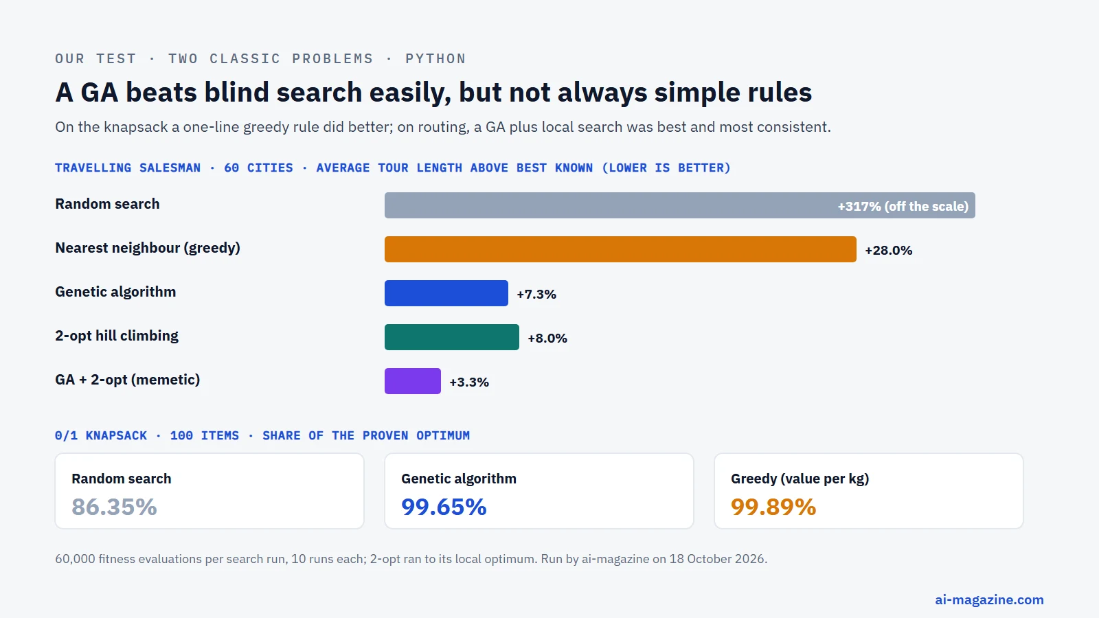
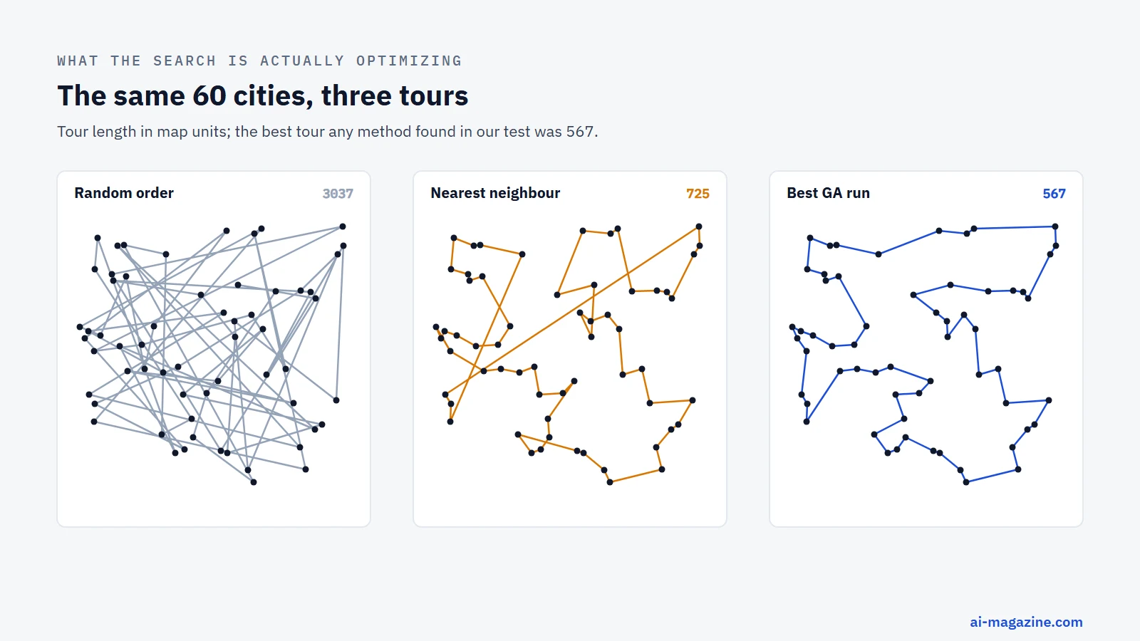
Problem 2: the travelling salesman. Find the shortest round trip through 60 random cities. Here there is no simple exact method at this size, so we compare each method with the best tour any of them found (length 567).
| Method | Average tour length above the best found | Spread over 10 runs |
|---|---|---|
| Random search | +317% | always terrible |
| Nearest neighbour (always go to the closest unvisited city) | +28.0% | deterministic |
| Genetic algorithm (order crossover, inversion mutation) | +7.3% | best run found the 567 tour; worst +13.9% |
| 2-opt hill climbing (keep untangling crossed edges) | +8.0% | best +2.7%, worst +13.9% |
| GA combined with 2-opt (a “memetic” algorithm) | +3.3% | +2.4% to +4.5% |
On routing, the plain GA was competitive with a classic local-search heuristic, and its best run found the shortest tour of the whole test. The clear winner, though, was the hybrid: a GA whose results are polished by local search was the best on average and by far the most consistent.
What this means in practice:
- Check the simple baseline first. If a greedy rule or an exact solver exists, use it; our knapsack is the classic example.
- GAs earn their place on messy search spaces, such as routes, schedules, layouts and designs, where there is no gradient and no good rule of thumb.
- Combine them with local search. In our test, adding 2-opt cut the average gap from 7.3% to 3.3% and made results far more predictable.
- Expect variance. The same GA, with different random seeds, landed anywhere from the best tour to 14% worse. Run it several times and keep the best.
Limits: two synthetic problem instances, one implementation each, 10 runs per method. Professional solvers (and better-tuned GAs) would do better; the point is the relative pattern, not the absolute numbers.
When to use a genetic algorithm, and when not to
Deciding whether to use a genetic algorithm (GA) comes down to the problem’s shape. If the landscape is smooth and differentiable, gradient descent wins. If it is rugged, discrete, or noisy, GAs shine.
Good fits:
- No gradient available: When you cannot calculate derivatives, or the function is black-box.
- Many local optima: a population explores many regions at once, so it is less likely to get stuck in one trap.
- Combinatorial problems: Scheduling, routing, and architecture search where the search space is discrete.
- Multi-objective optimization: NSGA-II (Deb et al., 2002) is a standard choice. It cuts complexity from O(MN³) to O(MN²) using fast non-dominated sort. It is elitist and needs no sharing parameter. It has 49,723 citations in OpenAlex, more than Holland’s 1975 book.
Poor fits:
- Smooth differentiable problems: Gradient methods are faster and more precise.
- Convex problems, or problems with a good exact or greedy method: dedicated solvers are faster and give guarantees; our knapsack test below is an example.
- High-dimensional continuous spaces: CMA-ES is better. It is derivative-free, invariant to monotone transformations, and needs few parameters to tune. It is ideal for 3–100 dimensions.
The No Free Lunch theorem (Wolpert & Macready, 1997) confirms this: no single algorithm works best for all problems. Elevated performance on one class means lower performance on another.
| Method | Best for | Needs a gradient? | Example |
|---|---|---|---|
| Genetic Algorithm | Discrete, multi-modal, black-box | No | NASA antenna design, crew scheduling |
| CMA-ES | Continuous, smooth but non-convex | No | Parameter tuning, robotics control |
| Gradient Descent | Smooth, differentiable, convex | Yes | Neural network training, linear regression |
| Greedy rule or exact solver | Problems with known structure | No | Knapsack by value per kilogram |
Genetic algorithm libraries
Choosing a library depends on your language and goal. DEAP is the classic Python choice, offering flexible building blocks. pymoo specializes in multi-objective optimization, implementing NSGA-II, NSGA-III, and CMA-ES. PyGAD is user-friendly for beginners. Jenetics is the go-to for Java developers. EvoTorch leverages PyTorch for GPU acceleration. OpenEvolve brings LLM-driven evolution to Python. pycma implements CMA-ES efficiently.
| Library | Language | What it is for | Version and licence |
|---|---|---|---|
| DEAP | Python | General-purpose EA framework | 1.4.4, LGPL-3.0 |
| PyGAD | Python | Simple GA and ML training | 3.9.2, BSD-3-Clause |
| pymoo | Python | Multi-objective optimization | 0.6.2, Apache-2.0 |
| Jenetics | Java | GA, GP, Grammatical Evolution | v9.1.0, Apache-2.0 |
| EvoTorch | Python/PyTorch | GPU-accelerated EA | 0.6.1, Apache-2.0 |
| OpenEvolve | Python | LLM-driven evolution (AlphaEvolve) | 0.4.0, Apache-2.0 |
| pycma | Python | CMA-ES for numerical optimization | 4.5.0, BSD-3 |
| FunSearch | Python | Reference code for LLM+EA | last push 2024-02-05, Apache-2.0 |
Start with DEAP if you want to understand the components. Move to pymoo if you need multi-objective results. Use OpenEvolve if you are experimenting with LLMs.
Advantages and limitations
Advantages:
- No gradient needed: Works on black-box functions.
- Global search: Avoids local optima better than gradient methods.
- Multi-objective: Handles competing goals natively (e.g., NSGA-II).
- Flexible representation: Works with strings, trees, graphs, and real numbers.
- Parallelizable: Each individual’s fitness can be evaluated independently.
Limitations:
- Slow convergence: Can be slower than gradient methods on smooth problems.
- Parameter tuning: Mutation/crossover rates need adjustment (pymoo recommends crossover 0.5–1.0, mutation 0.7–1.0).
- No guarantee: Does not guarantee the global optimum, only a good approximation.
- Computational cost: Evaluating complex fitness functions (like CFD simulations) can be expensive.
Frequently asked questions
What is a genetic algorithm in simple terms? A genetic algorithm is a search method inspired by natural evolution. It starts with a population of random solutions, evaluates their “fitness,” and selects the best ones to “breed” offspring. Mutation introduces small random changes. Over generations, the population evolves toward better solutions. It is a heuristic, not a guarantee of perfection.
What are the steps of a genetic algorithm?
- Initialize a random population.
- Evaluate fitness for each individual.
- Select parents based on fitness.
- Apply crossover to create offspring.
- Apply mutation to offspring.
- Replace the old population (or merge, as in elitism).
- Repeat until a termination condition is met.
Is a genetic algorithm machine learning? Not in the usual sense of learning from data. Genetic algorithms are an optimization method from evolutionary computation, a branch of AI. They are, however, widely used inside machine learning for hyperparameter tuning, feature selection and neural architecture search.
What is the difference between a genetic algorithm and genetic programming? Genetic algorithms typically optimize fixed-length strings or real numbers. Genetic programming evolves computer programs, usually represented as trees. Koza’s work popularized GP. GP can discover both the structure and parameters of a solution, whereas GAs usually optimize parameters within a fixed structure.
Are genetic algorithms still used in 2026? Yes. They are widely used in multi-objective optimization, neural architecture search, and algorithm discovery. AlphaEvolve and FunSearch show that GAs are evolving alongside LLMs. The 2026 Humies awards highlight ongoing human-competitive results. Libraries like pymoo and OpenEvolve are actively maintained.
What is a fitness function? The fitness function is the scorecard. It measures how good a solution is. It must be defined for your specific problem. For a traveling salesman problem, it might be the inverse of the total distance. For an antenna, it might be signal strength. The GA tries to maximize (or minimize) this value.