Machine Learning Algorithms: Types, How They Work and How to Choose One

Machine learning algorithms are procedures that learn patterns from data instead of following rules a programmer wrote by hand. Given examples, they fit a model that can classify an email as spam, predict a house price, group customers into segments or choose the next move in a game.

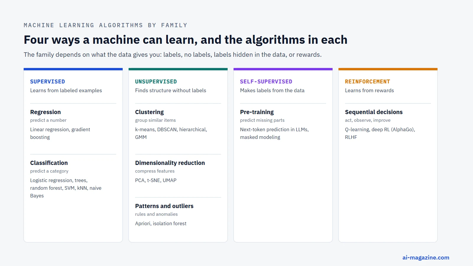
There are four main families: supervised learning (learning from labeled examples), unsupervised learning (finding structure in unlabeled data), semi- and self-supervised learning, and reinforcement learning (learning from rewards). This guide covers the algorithms that matter in each family: how they work, where each came from, what practitioners actually use, and what large benchmark studies say about which ones win. It ends with a decision guide and a scikit-learn example comparing seven algorithms, which we ran ourselves.

What is a machine learning algorithm?

To understand machine learning algorithms, you must distinguish between the algorithm itself and the model it produces. The algorithm is the procedure or “recipe” used to learn from data. For example, “grow decision trees on bootstrap samples” is an algorithm. The model is the trained result with fitted parameters. When you run the algorithm on a dataset, it minimizes a loss function on the training data. The goal is low error on new, unseen data, a property known as generalization. This generalization is measured on held-out test data or with cross-validation.

Training involves adjusting internal parameters to reduce the difference between predicted and actual values. Hyperparameters, however, are set before training begins and control the learning process itself, such as the depth of a decision tree or the learning rate of a neural network. Choosing the right hyperparameters is often as critical as choosing the algorithm.

Data is typically split into training and test sets. The training set teaches the algorithm. The test set evaluates how well the algorithm generalizes to new data. Cross-validation provides a more robust estimate of performance by repeatedly splitting the data into training and validation subsets. This helps detect overfitting, where a model performs well on training data but poorly on new data. Understanding this distinction between the recipe (algorithm) and the dish (model) is fundamental to debugging and improving your machine learning pipeline.

Types of machine learning algorithms

Machine learning algorithms are generally categorised by the type of feedback they receive during training. Supervised learning uses labelled data, where the correct output is known. Unsupervised learning works with unlabelled data, finding hidden structures. Semi-supervised and self-supervised learning use a mix of labelled and unlabelled data, or derive labels automatically from the input. Reinforcement learning involves an agent learning actions from rewards by trial and error.

Type	Learns from	Typical tasks	Example algorithms
Supervised	Labelled data	Classification, regression	Linear regression, decision trees, SVM, neural networks
Unsupervised	Unlabelled data	Clustering, dimensionality reduction, anomaly detection	k-means, PCA, DBSCAN, isolation forest
Semi-/Self-supervised	Partial or derived labels	Pre-training, scarce label scenarios	BERT, self-supervised contrastive learning
Reinforcement Learning	Rewards from environment	Sequential decision making, control	Q-learning, AlphaGo, RLHF for chatbots

Supervised learning is the most common form of machine learning in business applications. It is used when you have clear inputs and known outputs. The algorithm learns to map inputs to outputs by minimizing error on the labelled examples. This is the basis for most predictive modelling tasks in industry, from spam detection to price forecasting.

Unsupervised learning is used when you do not have labels. The algorithm finds patterns, clusters, or structures in the data. This is useful for exploratory data analysis, customer segmentation, or anomaly detection. The results are often harder to interpret because there is no ground truth to compare against.

Semi-supervised and self-supervised learning are increasingly important. Self-supervised learning, for example, is how large language models are trained. The algorithm generates its own labels from the data structure, allowing it to learn from vast amounts of unlabelled text or images. It is the first stage of training for modern language and vision models.

Reinforcement learning is used in dynamic environments where an agent must make a sequence of decisions. The agent learns by interacting with the environment and receiving rewards or penalties. It is used in robotics, game playing and the fine-tuning of chatbots. The agent learns a policy that maximises cumulative reward over time.

Supervised learning algorithms

Supervised learning algorithms predict a target variable based on input features. They are divided into classification, where the output is a category, and regression, where the output is a number. Each algorithm has specific strengths, weaknesses, and origins. Understanding these helps you choose the right tool for your problem.

Linear regression

Linear regression is the simplest supervised algorithm. It models the relationship between a dependent variable and one or more independent variables as a linear equation. The algorithm learns the coefficients that minimise the sum of squared errors between predicted and actual values. This is known as the method of least squares.

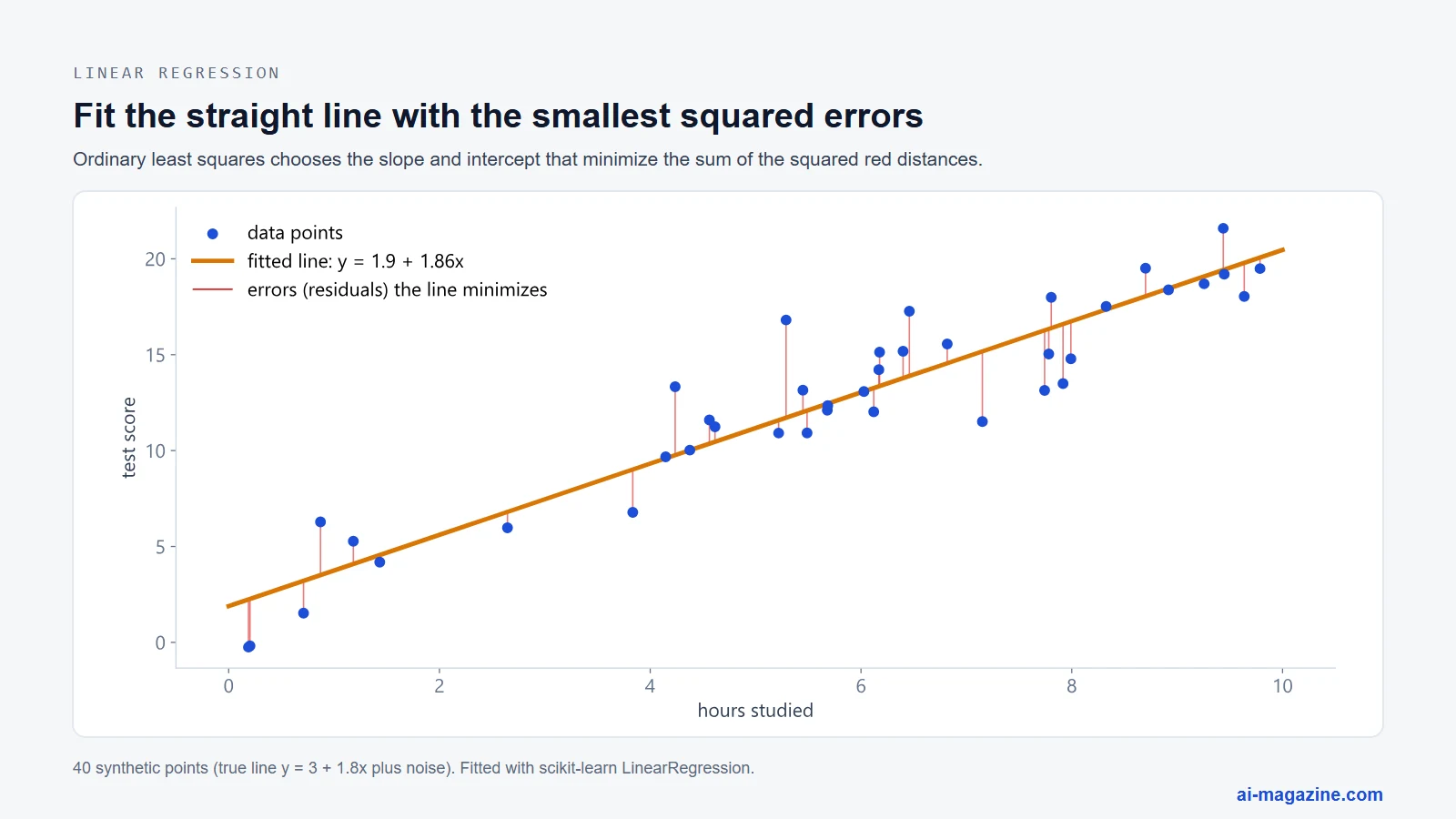
The method was published by Adrien-Marie Legendre in 1805. Carl Friedrich Gauss claimed in 1809 that he had been using it since 1795, which led to a priority dispute. Despite its age, linear regression remains a baseline for many problems. It is fast, easy to interpret, and provides a clear understanding of how each feature affects the target variable.

Linear regression is good at handling linear relationships and provides a strong baseline for more complex models. However, it assumes a linear relationship between features and the target. If the relationship is non-linear, linear regression will perform poorly. It is also sensitive to outliers, which can skew the coefficients.

Use linear regression when you need a simple, interpretable model, when the relationship between features and target is approximately linear, or when you need a baseline to compare against more complex models. It is also useful when computational resources are limited.

Logistic regression

Logistic regression is used for binary classification. It models the probability that a given input belongs to a particular class. Instead of predicting a continuous value, it predicts a probability between 0 and 1. This probability is passed through a logistic function, also known as the sigmoid function, to produce a binary output.

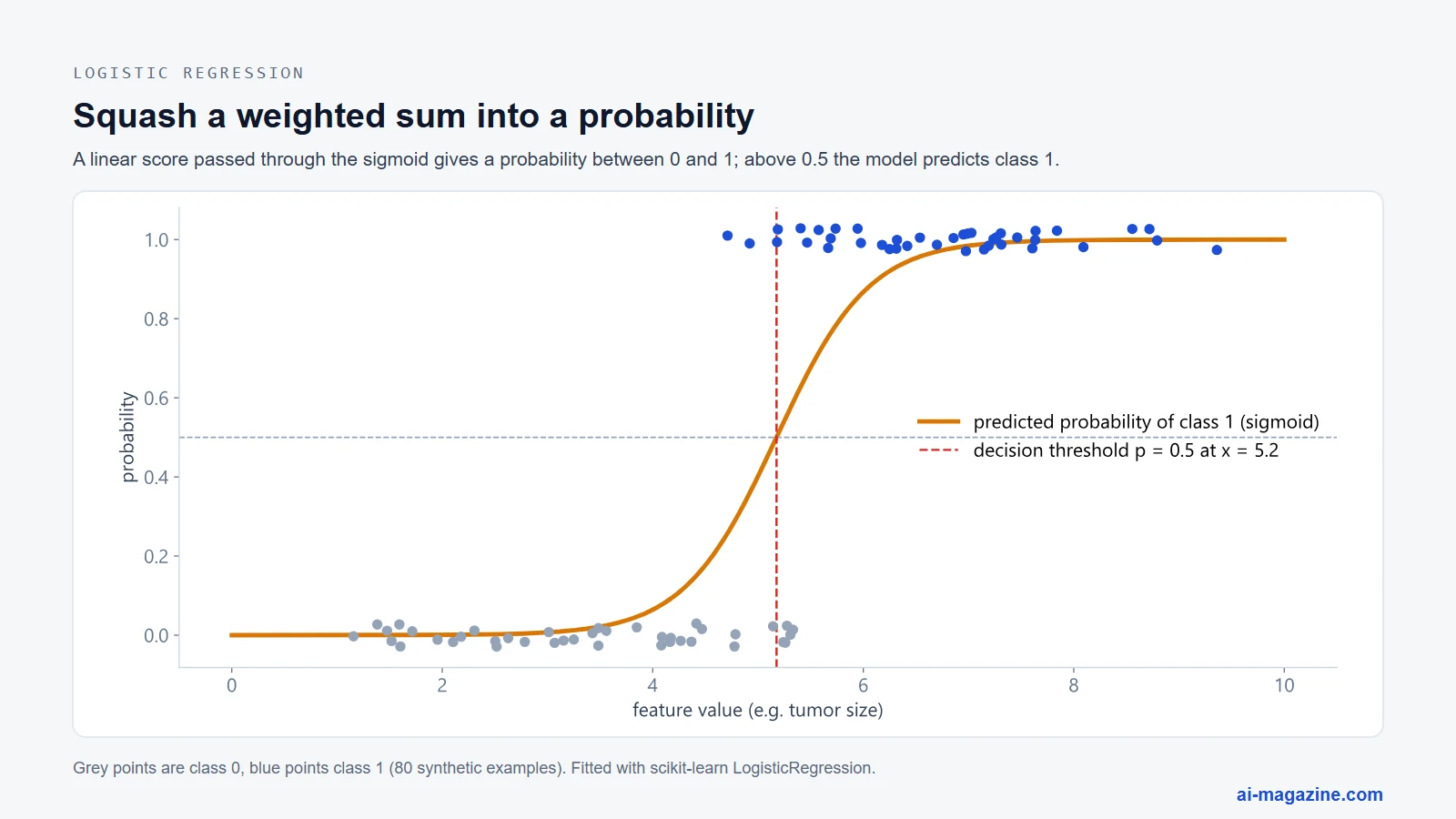
The algorithm was formalised by D.R. Cox in the paper “The Regression Analysis of Binary Sequences”, published in the Journal of the Royal Statistical Society Series B in 1958. Cox’s work provided a rigorous statistical foundation for logistic regression, which has since become a standard tool in classification.

Logistic regression is good at providing probabilistic outputs, which are useful for decision-making. It is also computationally efficient and easy to interpret. The coefficients indicate the direction and magnitude of the effect of each feature on the log-odds of the target class. However, it assumes a linear relationship between the features and the log-odds of the target. It may struggle with complex, non-linear patterns.

Use logistic regression when you need a simple, interpretable classifier, when the decision boundary is approximately linear, or when you need probabilistic outputs. It is also useful as a baseline for more complex classifiers.

Decision trees

Decision trees split the data recursively based on feature values to create a tree-like model of decisions. Each internal node represents a test on a feature, each branch represents the outcome of the test, and each leaf node represents a class label or regression value. The algorithm selects the feature that best splits the data at each step, often using metrics like Gini impurity or information gain.

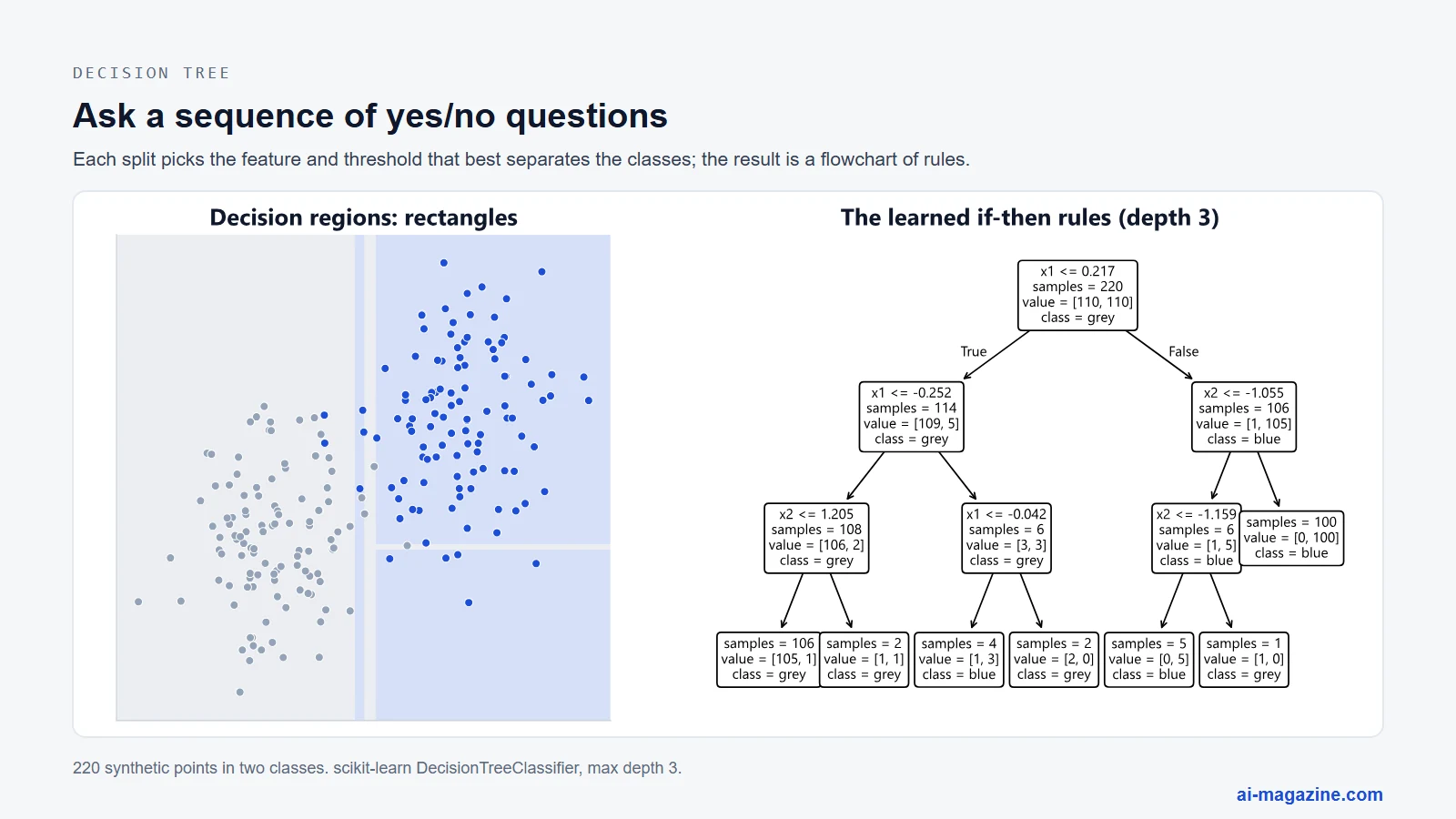
The Classification and Regression Trees (CART) algorithm was developed by Leo Breiman, Jerome Friedman, Richard Olshen, and Charles Stone, and published in their 1984 book. Ross Quinlan later developed the ID3 algorithm, published in the Machine Learning journal in 1986, and its successor C4.5, published in his 1993 book. These algorithms laid the foundation for modern decision tree learning.

Decision trees are good at handling non-linear relationships and mixed data types. They are easy to interpret and visualise, making them useful for explaining model decisions. However, they are prone to overfitting, especially when the tree is deep. Small changes in the data can lead to significantly different trees, making them unstable.

Use decision trees when you need an interpretable model, when the data has non-linear relationships, or when you want to visualise the decision process. They are also useful as a baseline for ensemble methods.

Random forests

Random forests are an ensemble method that combines multiple decision trees to improve performance and reduce overfitting. Each tree is trained on a bootstrap sample of the data, and a random subset of features is considered at each split. The final prediction is the average (for regression) or majority vote (for classification) of all trees.

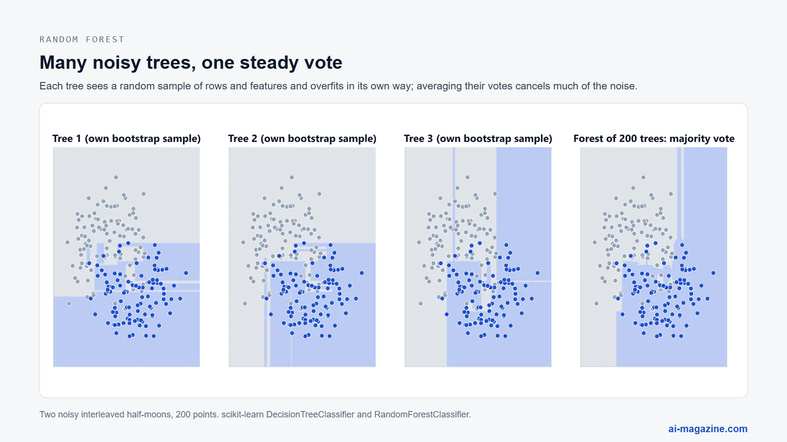
The algorithm was introduced by Leo Breiman in the paper “Random Forests”, published in Machine Learning in October 2001. Averaging many decorrelated trees removes most of the instability of a single tree.

Random forests are good at handling high-dimensional data and reducing overfitting. They are robust to noise and outliers, and they provide estimates of feature importance. However, they are less interpretable than single decision trees, as the ensemble of trees is harder to visualise. They can also be slower to train and predict than single trees.

Use random forests when you need a robust, accurate model, when the data is high-dimensional, or when you want to reduce overfitting. They are also useful when interpretability is less critical than accuracy.

Gradient boosting (XGBoost, LightGBM, CatBoost)

Gradient boosting builds an ensemble of weak learners, typically decision trees, sequentially. Each new tree is trained to correct the errors of the previous ensemble. The algorithm minimizes a differentiable loss function by adding new trees that fit the residual errors. This approach often achieves high accuracy and is widely used in machine learning competitions.

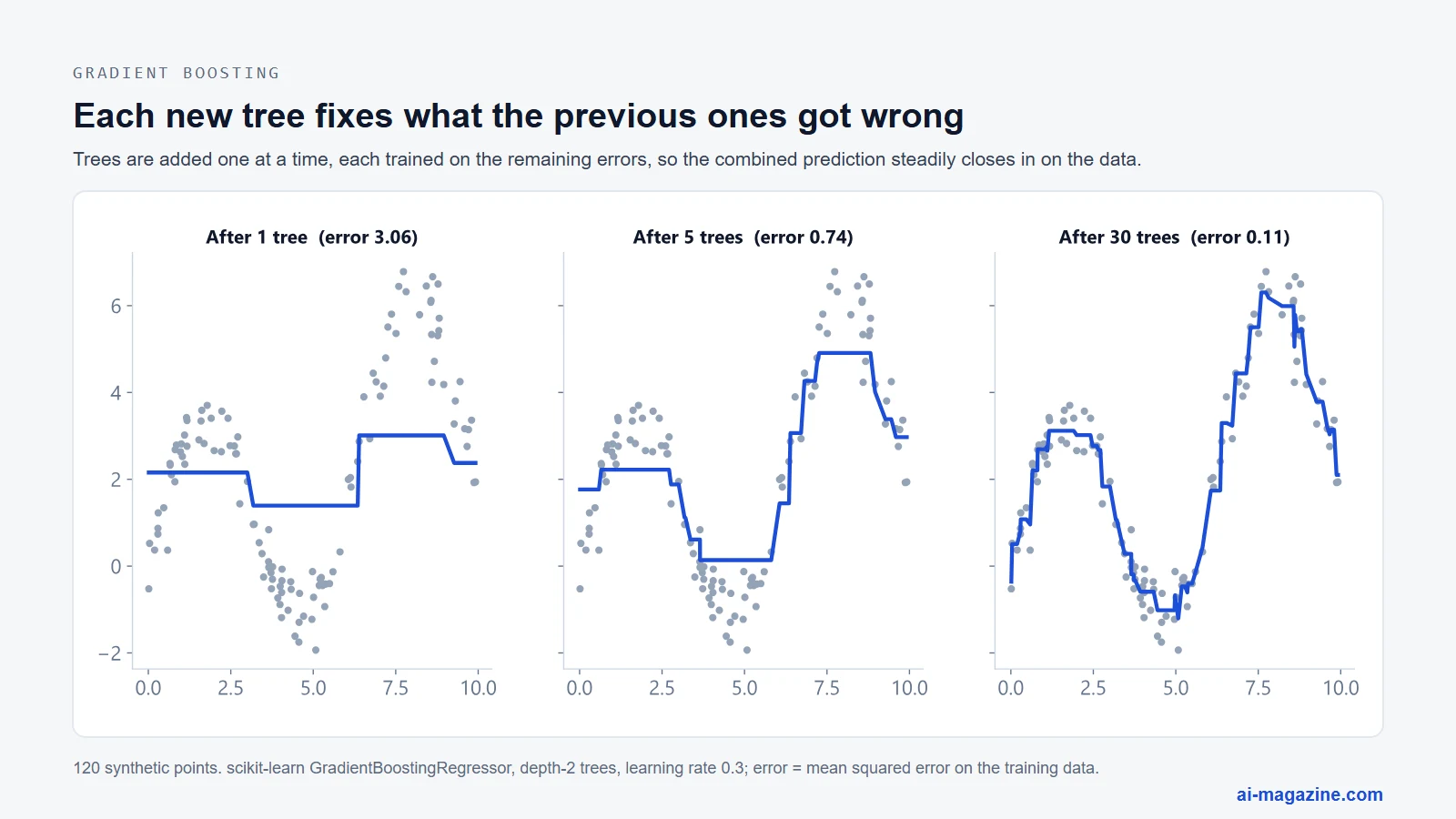
Jerome Friedman published “Greedy function approximation: A gradient boosting machine” in the Annals of Statistics in 2001, laying the theoretical foundation. Later, Tianqi Chen and Carlos Guestrin introduced XGBoost at KDD in 2016. Their paper noted that “among the 29 challenge winning solutions published at Kaggle’s blog during 2015, 17 solutions used XGBoost”. In KDDCup 2015, XGBoost was used by every winning team in the top-10. Microsoft’s LightGBM was presented at NeurIPS in 2017, and its paper reports training “up to over 20 times” faster than conventional gradient-boosted decision trees. Yandex’s CatBoost, presented at NeurIPS in 2018, introduced ordered boosting and native handling of categorical features.

Gradient boosting is good at achieving state-of-the-art accuracy on tabular data. It handles missing values well and can incorporate complex feature interactions. However, it can be prone to overfitting if not regularised properly. Trees are built one after another, so training cannot be spread across trees the way a random forest’s can, and results depend more on tuning (learning rate, number of trees, depth).

Use gradient boosting when you need high accuracy on tabular data with thousands of rows or more, or when you have missing values and categorical features. XGBoost, LightGBM, and CatBoost are the leading implementations.

Support vector machines (SVM)

Support vector machines find a hyperplane that maximises the margin between classes in a high-dimensional space. For non-linearly separable data, SVMs use kernel functions to map the data into a higher-dimensional space where it becomes linearly separable. The algorithm seeks the optimal boundary that separates the classes with the largest possible gap.

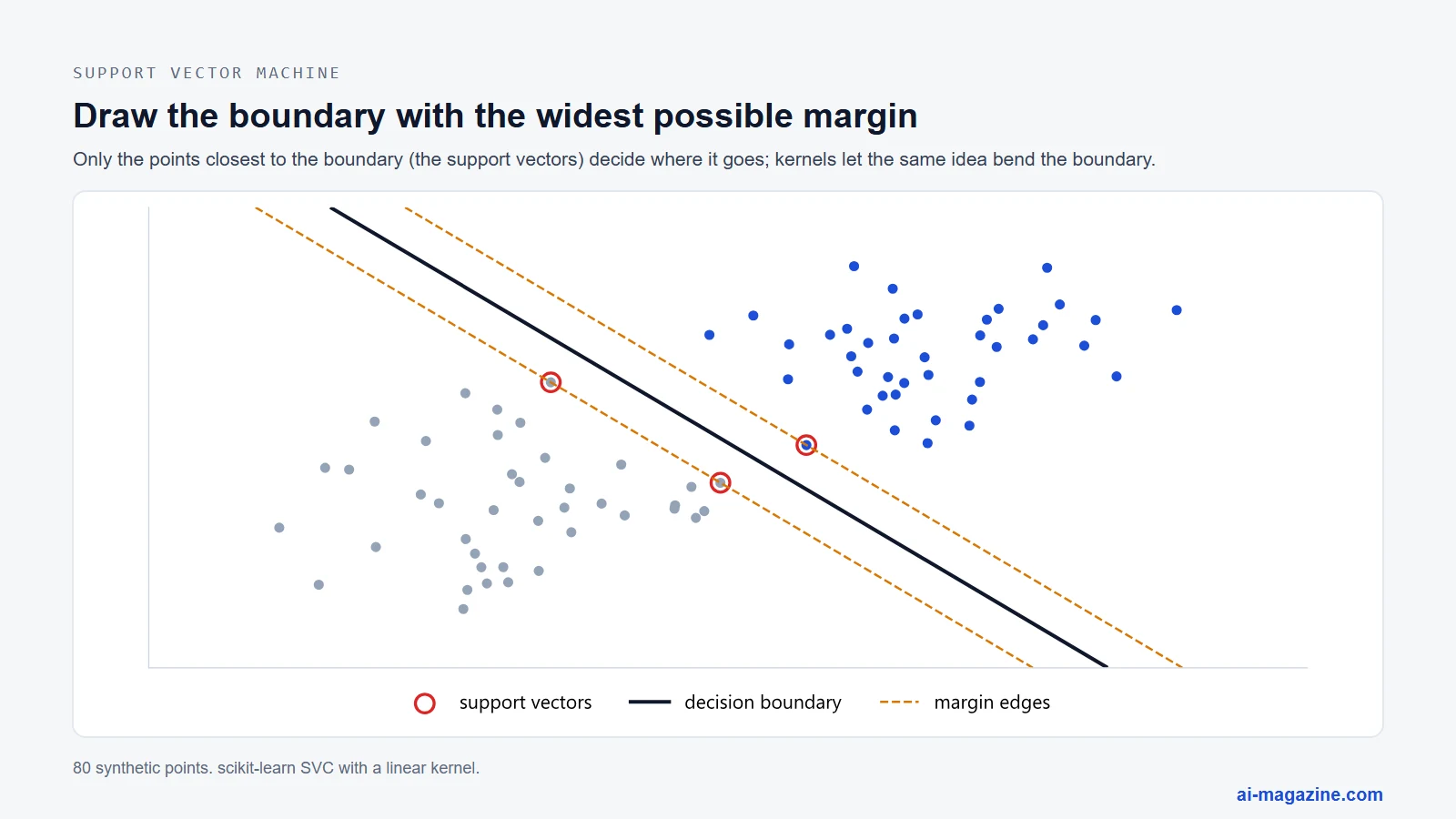
Corinna Cortes and Vladimir Vapnik published “Support-vector networks” in Machine Learning in 1995. Their work popularised SVMs and provided a theoretical basis for their generalization performance. Through the late 1990s and 2000s SVMs were a default choice for text classification and many recognition tasks, before deep learning took over images.

SVMs are good at handling high-dimensional spaces and non-linear relationships through kernels. They are effective when the number of dimensions exceeds the number of samples. However, they can be computationally expensive for large datasets, as the training complexity is often between O(n²) and O(n³). They are also sensitive to the choice of kernel and hyperparameters.

Use SVMs when you have a clear margin of separation, when the data is high-dimensional, or when the dataset is not too large. They are also useful for text classification and bioinformatics applications.

k-nearest neighbors (kNN)

k-nearest neighbors is a non-parametric algorithm that classifies a data point based on the majority class of its k nearest neighbours in the feature space. The algorithm calculates the distance between the query point and all training points, then selects the k closest points. The class label is determined by the majority vote of these neighbours.

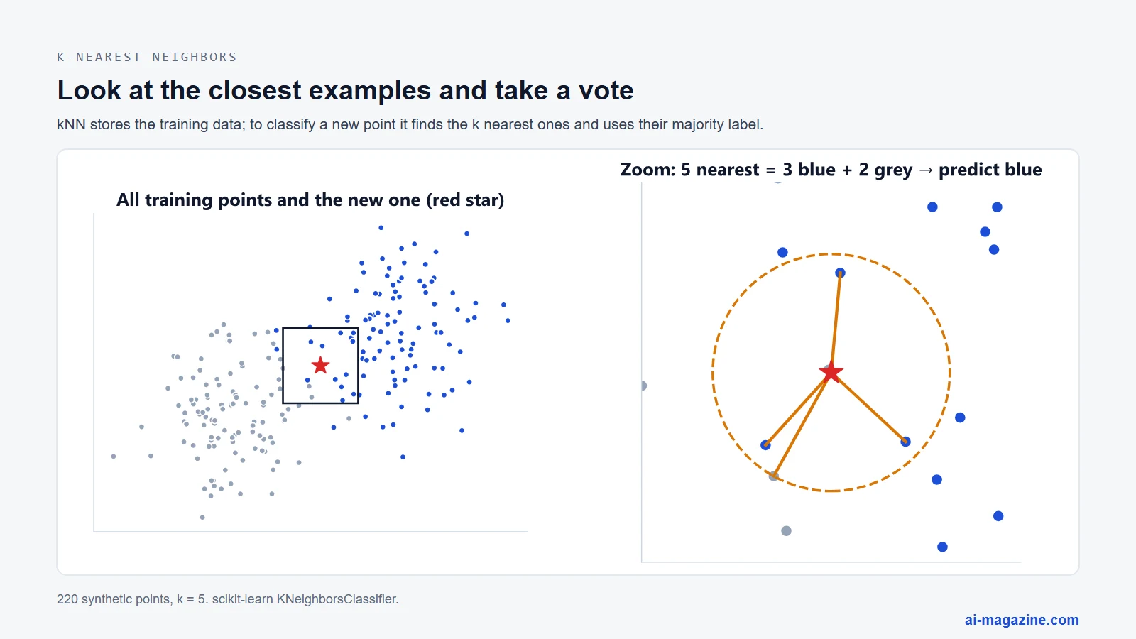
The concept was first introduced by Evelyn Fix and Joseph Hodges in a US Air Force School of Aviation Medicine report in February 1951, though it was not published until a 1989 reprint. Thomas Cover and Peter Hart formalised the algorithm in “Nearest neighbor pattern classification”, published in IEEE Transactions on Information Theory in 1967.

kNN is good for simple, intuitive classification and can handle multi-class problems easily. It requires no training phase, as the entire dataset is stored. However, it is slow at prediction time, as it must calculate distances to all training points. It is also sensitive to the scale of the features and the choice of k.

Use kNN when you have a small dataset, when the decision boundary is irregular, or when similar items should get similar answers, as in simple recommendation and anomaly detection. Always scale the features first.

Naive Bayes

Naive Bayes is a probabilistic classifier based on Bayes’ theorem, assuming that features are conditionally independent given the class label. Despite the strong independence assumption, it often performs well, especially in text classification. The algorithm calculates the probability of each class given the features and selects the class with the highest probability.

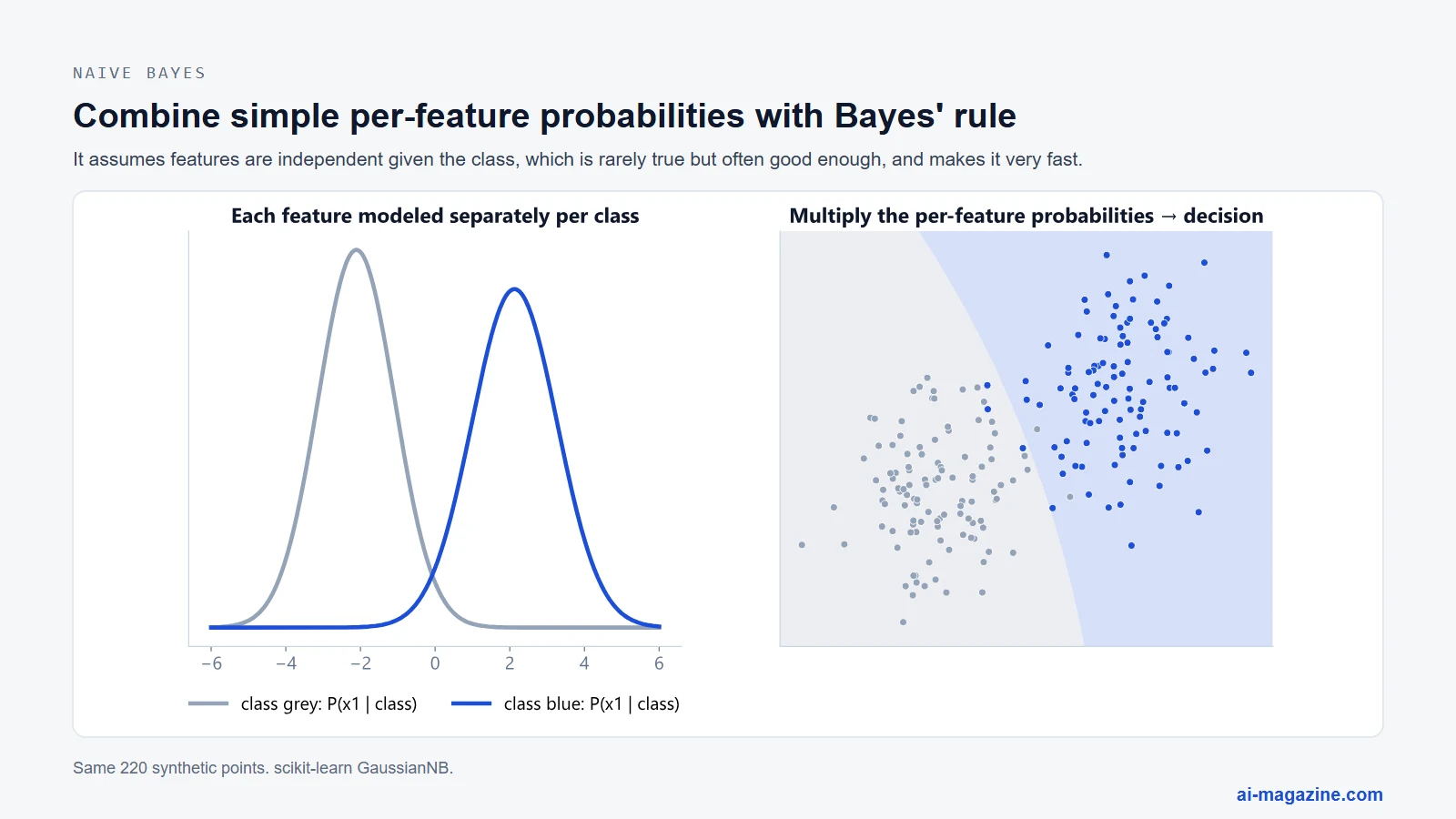
Maron’s 1961 paper “Automatic Indexing” in the Journal of ACM is commonly cited as an early naive-Bayes text classifier. Later, Sahami, Dumais, Heckerman, and Horvitz used it for spam filtering in a 1998 AAAI workshop paper. Paul Graham’s 2002 essay “A Plan for Spam” reported that his Bayesian filter missed “less than 5 per 1000 spams, with 0 false positives”.

Naive Bayes is good for text classification, spam filtering, and real-time prediction due to its speed. It works well with high-dimensional data and requires little training data. However, the independence assumption is often violated in real-world data, which can reduce accuracy. It also cannot learn feature interactions.

Use Naive Bayes for text classification, spam filtering, or when you need a fast, simple classifier. It is also useful when data is high-dimensional and features are relatively independent.

Neural networks

Neural networks are composed of layers of interconnected nodes (neurons) that process information. Each connection has a weight, which is adjusted during training to minimise error. Training uses backpropagation to calculate gradients and gradient descent and update weights. Neural networks can model complex, non-linear relationships and are the foundation of deep learning.

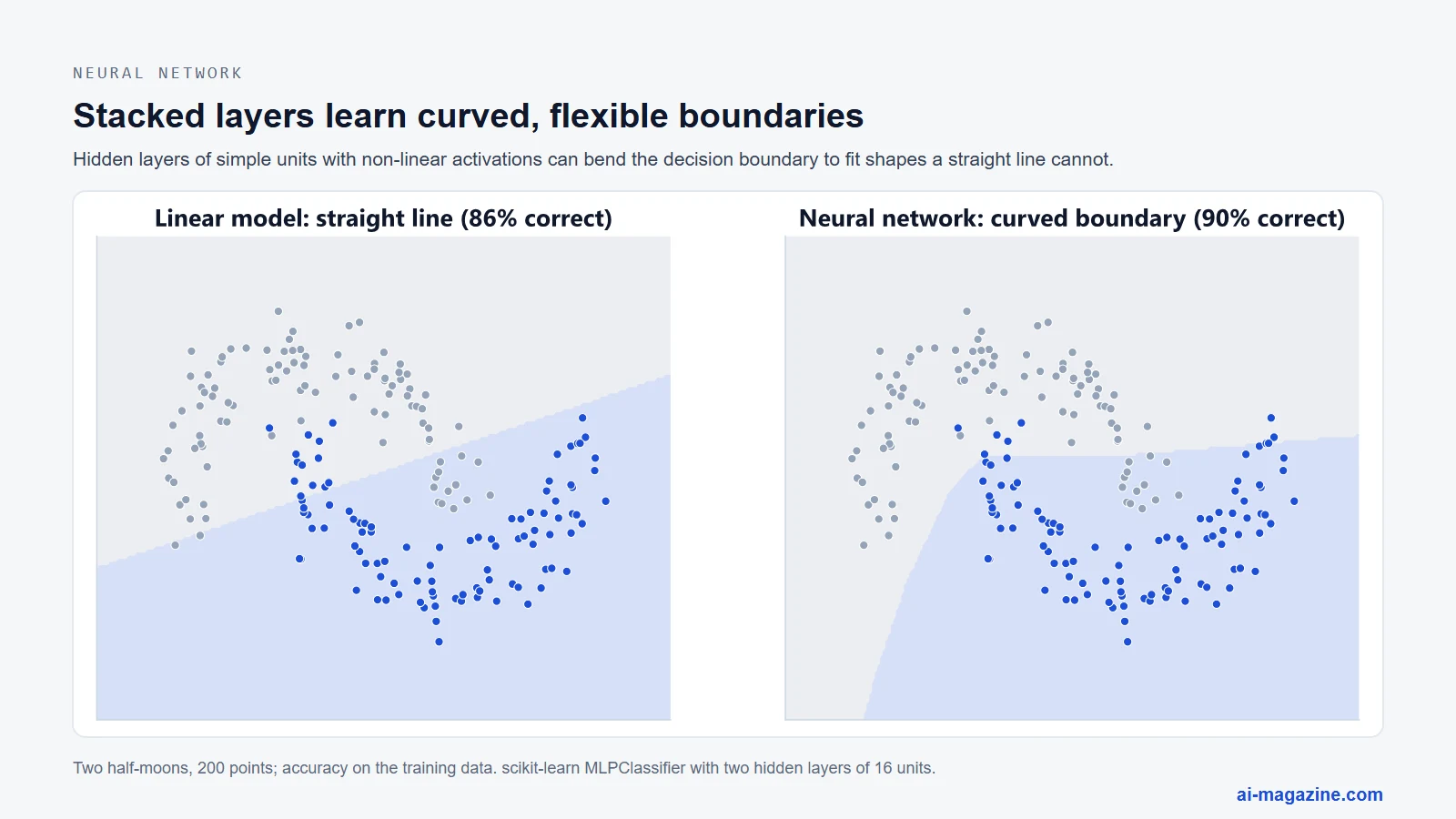
Frank Rosenblatt introduced the perceptron, the first trainable artificial neuron, in Psychological Review in 1958. David Rumelhart, Geoffrey Hinton, and Ronald Williams published the backpropagation algorithm in Nature in October 1986, enabling the training of multi-layer networks. The transformer architecture, introduced in “Attention Is All You Need” in June 2017, now underlies large language models and many vision models (how attention works).

Neural networks are good at handling unstructured data like images, audio, and text. They can learn hierarchical features and achieve state-of-the-art performance in many domains. However, they require large amounts of data and computational resources. They are also often considered black boxes, making them harder to interpret than linear models or decision trees.

Use neural networks for image, audio, or text data, when you have large datasets, or when you need to capture complex patterns. They are also essential for deep learning applications like language models and computer vision.

Supervised algorithms compared

The following table summarises the key characteristics of the supervised learning algorithms discussed.

Algorithm	Task	Strengths	Weaknesses	Interpretability
Linear Regression	Regression	Simple, fast, interpretable	Assumes linearity, sensitive to outliers	High
Logistic Regression	Classification	Probabilistic, fast, interpretable	Assumes linearity in log-odds	High
Decision Trees	Classification/Regression	Interpretable, handles non-linearity	Prone to overfitting, unstable	High
Random Forests	Classification/Regression	Robust, reduces overfitting, accurate	Less interpretable, slower prediction	Medium
Gradient Boosting	Classification/Regression	High accuracy, handles missing data	Prone to overfitting, slow training	Low
SVM	Classification/Regression	Effective in high dimensions, robust	Slow for large datasets, sensitive to kernel	Low
kNN	Classification/Regression	Simple, no training phase	Slow prediction, sensitive to scale	Medium
Naive Bayes	Classification	Fast, works well with text	Assumes feature independence	High
Neural Networks	Classification/Regression	Handles unstructured data, high accuracy	Requires large data, black box	Low

Unsupervised learning algorithms

Unsupervised learning works without labeled outcomes and looks for structure in the data itself. Since there is no target variable to minimise a loss function against, evaluation often relies on internal metrics like cluster cohesion or reconstruction error. These methods are essential for exploratory data analysis, feature engineering, and compressing high-dimensional data into manageable forms.

k-means clustering

K-means is the best-known clustering algorithm. Stuart Lloyd described it in a Bell Labs manuscript dated 31 July 1957, which was published only in 1982; James MacQueen gave it the name “k-means” in 1967. The algorithm works by partitioning data into $k$ clusters by minimising the within-cluster sum of squared distances to the cluster centroid. It assigns each data point to the nearest centroid, recalculates centroids based on the mean of assigned points, and repeats until convergence.

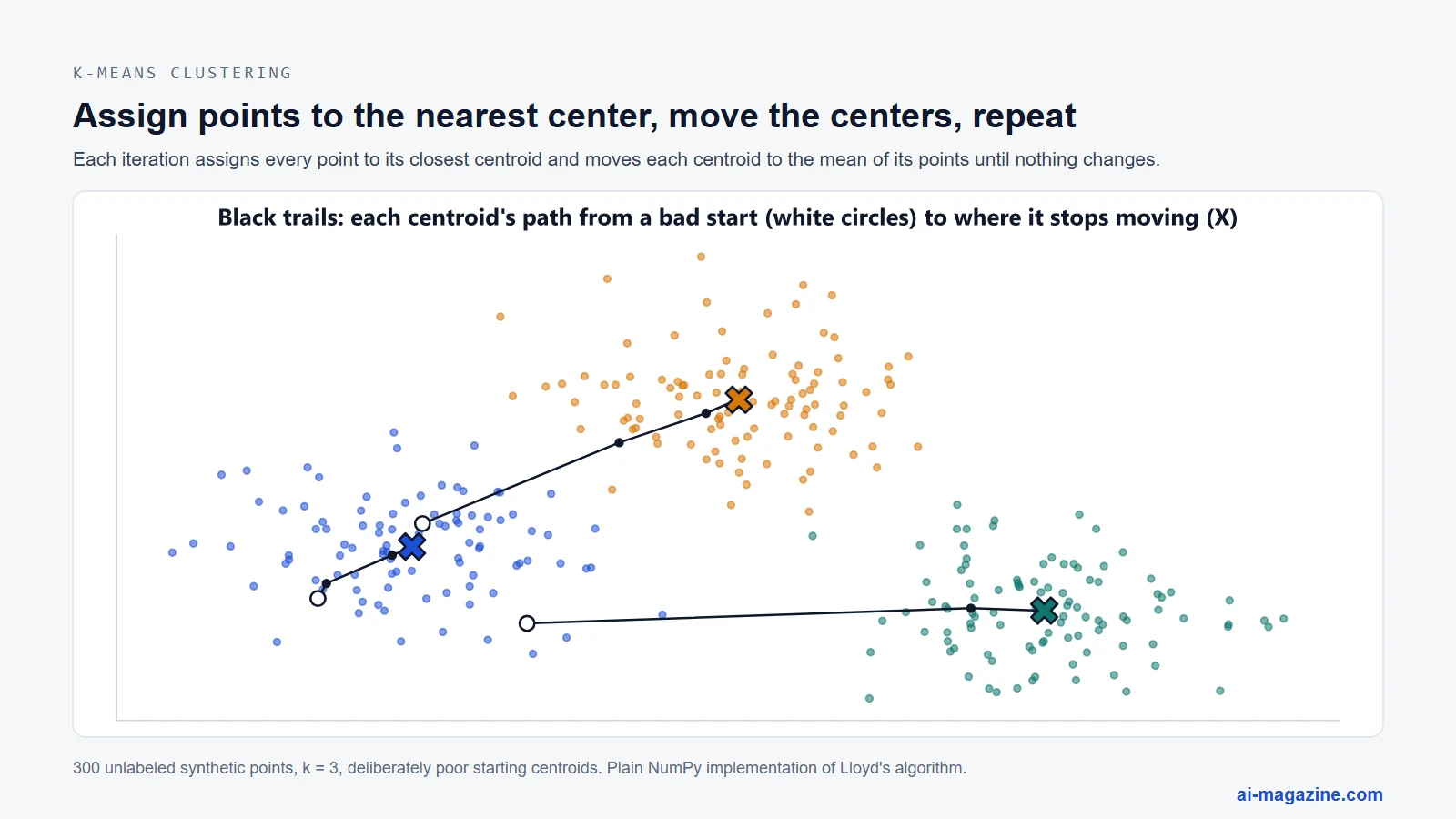
This algorithm is ideal for segmenting customers, compressing images, or grouping similar text documents. Its primary weakness is that it assumes clusters are spherical and of similar size. It also requires the number of clusters ($k$) to be specified in advance. If the data has irregular shapes or vastly different densities, k-means will struggle to represent the structure accurately.

Hierarchical clustering and DBSCAN

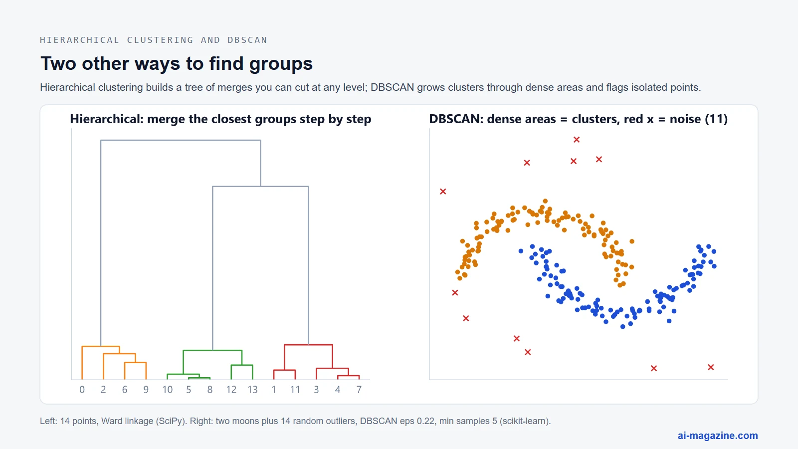
Hierarchical clustering builds a tree of clusters rather than a flat partition. It either merges the closest pairs of clusters (agglomerative) or splits the largest cluster (divisive) until a stopping criterion is met. This method provides a dendrogram, allowing data scientists to visualise relationships at multiple scales without pre-defining the number of clusters.

Density-Based Spatial Clustering of Applications with Noise (DBSCAN), introduced by Ester, Kriegel, Sander, and Xu at KDD in 1996, takes a different approach. It defines clusters as regions of high density separated by regions of low density. DBSCAN identifies core points that have at least a minimum number of points within a specified radius. Crucially, it can find clusters of arbitrary shape and explicitly marks points that do not belong to any cluster as noise. Its paper notes that DBSCAN outperformed the CLARANS algorithm by a factor of more than 100 in terms of efficiency. However, DBSCAN struggles when clusters have significantly varying densities or when the dataset is very large, as its computational complexity can become prohibitive without spatial indexing.

Gaussian mixture models

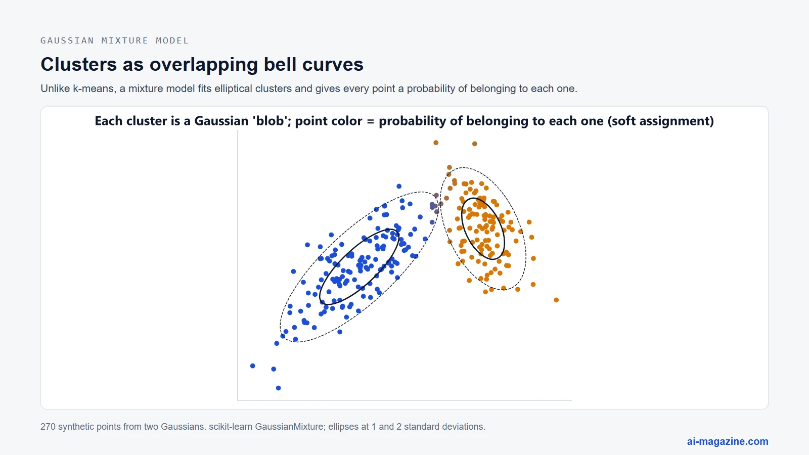
Gaussian mixture models (GMMs) generalise k-means by assuming that all data points are generated from a mixture of a finite number of Gaussian distributions with unknown parameters. Unlike k-means, which assigns a point to a single cluster, GMMs provide the probability that a point belongs to each cluster. This soft clustering is more realistic for data with overlapping groups. The parameters are typically estimated using the Expectation-Maximisation algorithm. GMMs are useful for anomaly detection and density estimation but require careful tuning of the number of components to avoid overfitting the noise in the data.

Principal component analysis (PCA)

Principal component analysis is a dimensionality reduction technique, not a clustering algorithm. Karl Pearson introduced PCA in 1901, and Harold Hotelling formalised it in 1933. PCA works by projecting data onto a new coordinate system defined by the eigenvectors of the data’s covariance matrix. These new axes, or principal components, are orthogonal and ordered by the amount of variance they explain. By keeping only the top components, you can reduce the dimensionality of the dataset while preserving as much information as possible.

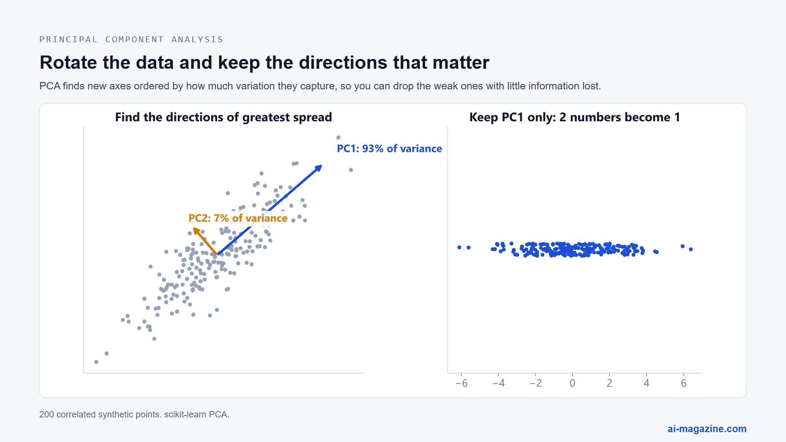
PCA is widely used for visualising high-dimensional data, removing multicollinearity before regression, and noise reduction. Its main limitation is that it is a linear method; it cannot capture complex non-linear relationships in the data. Additionally, the principal components are linear combinations of the original features, which can make them difficult to interpret in domains where feature meaning is critical.

t-SNE and UMAP

When visualising high-dimensional data, linear methods like PCA often fail to preserve local structures. t-Distributed Stochastic Neighbor Embedding (t-SNE), introduced by van der Maaten and Hinton in 2008, addresses this by modelling pairwise similarities between points in high-dimensional and low-dimensional spaces. It minimizes the divergence between these similarity distributions, making it excellent for revealing local clusters in 2D or 3D visualisations. However, t-SNE is computationally expensive and stochastic, meaning different runs can produce different layouts. It also does not preserve global structure well, so distances between distant clusters are not meaningful.

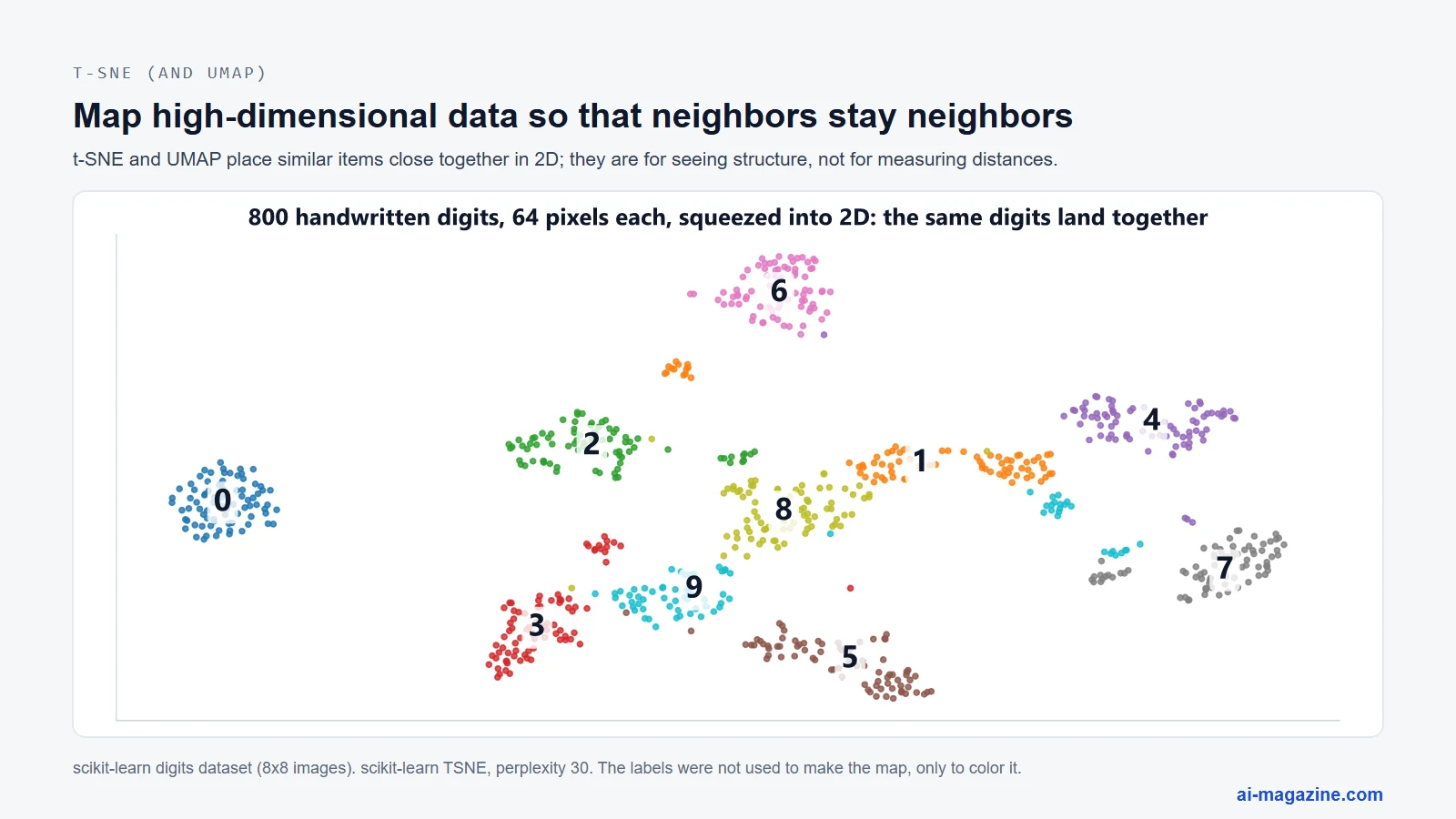
Uniform Manifold Approximation and Projection (UMAP), developed by McInnes, Healy, and Melville in February 2018, uses similar topological principles but is significantly faster. Its authors report that it is faster than t-SNE and keeps more of the data’s global structure, and it has become a common alternative for visualizing embeddings.

Association rules and anomaly detection

Association rules, such as the Apriori algorithm, identify frequent co-occurring items in transactional data. This is the backbone of market-basket analysis, revealing that customers who buy bread are likely to also buy butter. These rules are straightforward to interpret but can generate a vast number of uninteresting rules unless constrained by minimum support and confidence thresholds.

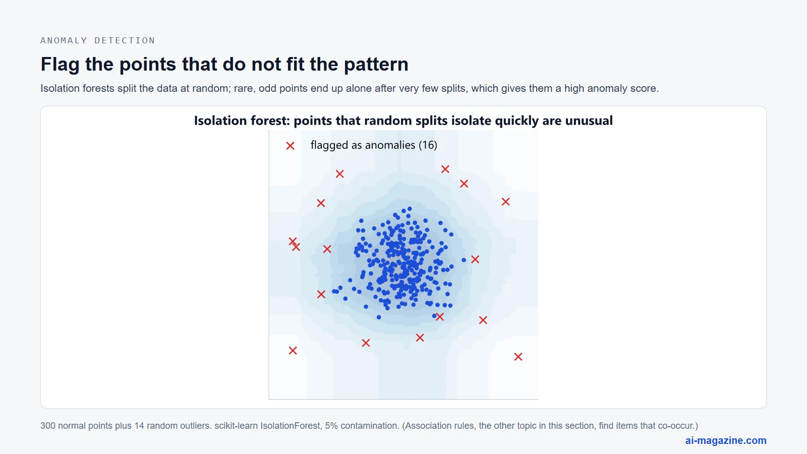
Anomaly detection methods, such as isolation forests, identify rare items or events that differ significantly from the majority. Isolation forests work by randomly partitioning data into trees; anomalies are isolated quicker than normal points because they are few and distinct. These detectors are crucial for fraud detection, network intrusion detection, and quality control in manufacturing.

Reinforcement learning algorithms

Reinforcement learning (RL) differs from supervised and unsupervised learning by focusing on decision-making. An agent interacts with an environment, taking actions that transition the environment to a new state. The environment responds with a reward signal, indicating how good or bad the action was. The agent’s goal is to learn a policy—a mapping from states to actions—that maximises the cumulative reward over time. This trial-and-error learning process is fundamental to robotics, game playing, and resource management.

Q-learning

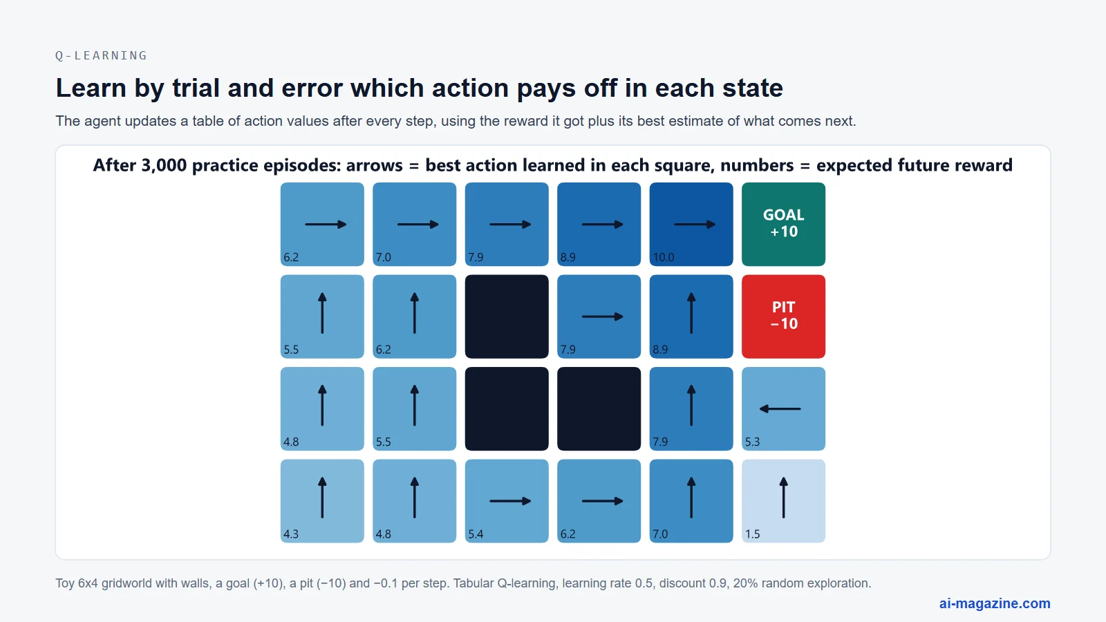
Q-learning is one of the earliest and most influential model-free RL algorithms. Chris Watkins introduced it in his 1989 PhD thesis, “Learning from Delayed Rewards,” and later published it with Peter Dayan in 1992. The algorithm maintains a Q-table that estimates the expected future reward for taking a specific action in a specific state. It updates these values using the Bellman equation, balancing immediate rewards with the expected value of future states. Q-learning is off-policy, meaning it can learn the value of the optimal policy independently of the agent’s actions. While foundational, tabular Q-learning does not scale to environments with large or continuous state spaces, leading to the development of deep RL.

Deep RL and AlphaGo/AlphaZero

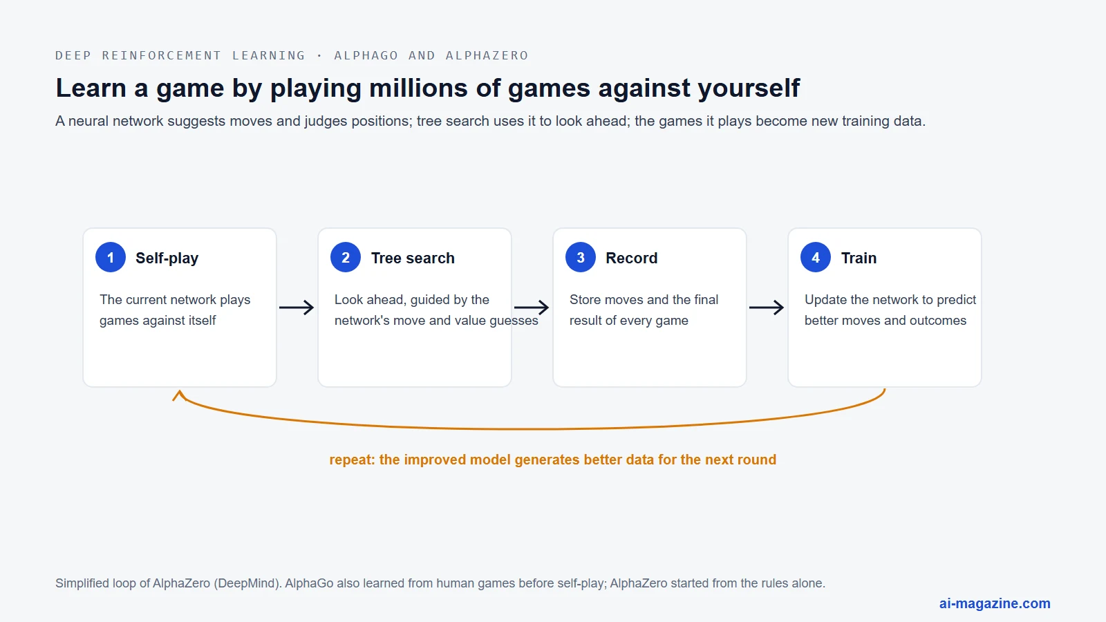
Deep reinforcement learning combines neural networks with RL to handle high-dimensional inputs like images. A landmark achievement was AlphaGo, developed by DeepMind. Published in Nature in January 2016, AlphaGo used neural networks trained by supervised learning on expert games and refined through reinforcement learning via self-play. It achieved a 99.8% winning rate against other Go programs and beat Lee Sedol, one of the strongest players in the world, 4–1 in Seoul in March 2016.

AlphaZero, described in Science in December 2018, took this further. Starting from random play and given no domain knowledge except the game rules, it learned chess, shogi and Go and beat the world-champion programs in all three. One algorithm mastered three games without any human game data.

RLHF for chatbots

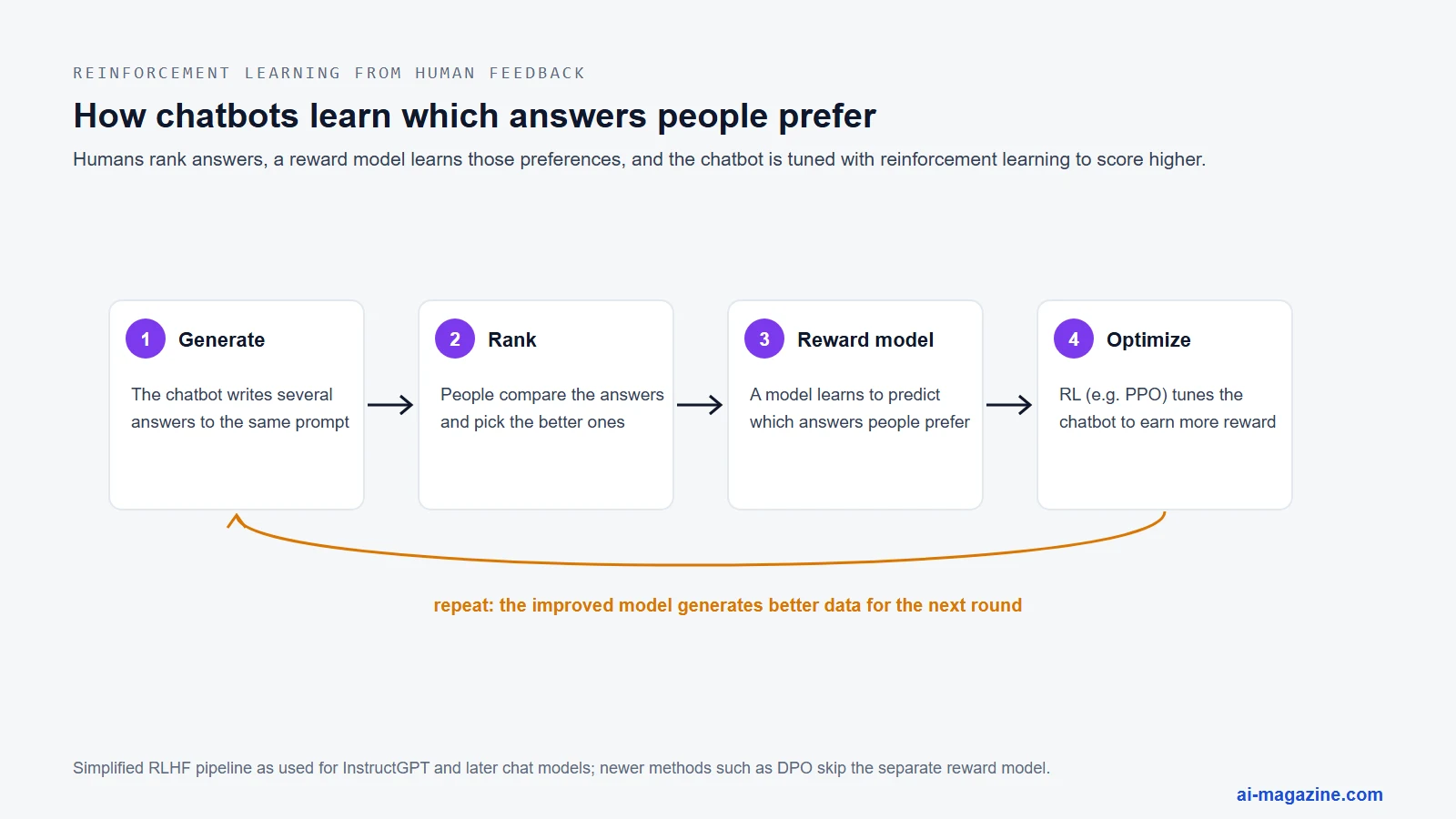
Reinforcement learning from human feedback (RLHF) has become the standard for fine-tuning large language models. After a model is pre-trained on vast text data, it is fine-tuned using human preferences. Human raters rank different model outputs, and a reward model is trained on these rankings. The language model is then optimised using RL to maximise the reward from the reward model. This process aligns the model’s outputs with human values, improving helpfulness and reducing toxicity.

Which algorithms actually win? What the evidence says

There is no universal winner in machine learning. The choice of algorithm depends heavily on the data type, size, and structure. Evidence from large-scale benchmarks and practitioner surveys provides a clearer picture than hype.

What data scientists use

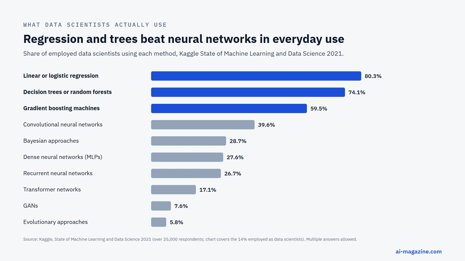
According to the Kaggle “State of Machine Learning and Data Science 2021” report, which surveyed over 25,000 respondents, the most used methods among the 14% employed as data scientists are linear or logistic regression (80.3%), decision trees or random forests (74.1%), and gradient boosting machines (59.5%). Convolutional neural networks (39.6%) and Bayesian approaches (28.7%) follow. Dense neural networks (MLPs) were used by 27.6%, recurrent neural networks by 26.7%, and transformer networks by 17.1%. Generative adversarial networks (GANs) were used by 7.6%, and evolutionary approaches by 5.8%. The same report found scikit-learn was used by over 80% of data scientists. The simple, decades-old methods are still the everyday workhorses.

The 179-classifier study

A comprehensive study by Fernández-Delgado et al., published in the Journal of Machine Learning Research in 2014, tested 179 classifiers from 17 families across 121 real-world datasets. Random forest came out on top: it reached on average 94.1% of the best accuracy achieved on each dataset, and more than 90% of it on 84.3% of the datasets. A Gaussian-kernel support vector machine came in second at 92.3%, but the difference was statistically insignificant. The practical lesson: a well-configured random forest or SVM is a hard baseline to beat.

Trees vs deep learning on tabular data

On tabular data, tree-based models often outperform deep neural networks. Grinsztajn, Oyallon, and Varoquaux published a study at NeurIPS 2022 using 45 datasets. They found that tree-based models like XGBoost and random forests remained state of the art on medium-sized datasets of about 10,000 samples, even without accounting for their superior speed. Their analysis, which included 20,000 compute-hours of hyperparameter search, revealed that neural networks are less robust to uninformative features and struggle to learn irregular functions common in tabular data.

Shwartz-Ziv and Armon (2021) reinforced this, noting that XGBoost outperforms deep models across many datasets and requires much less tuning. They found that an ensemble of deep models plus XGBoost achieved the best results, suggesting that trees and neural networks capture different patterns.

XGBoost’s dominance is also visible in competition data. The original XGBoost paper, published at KDD 2016 by Chen and Guestrin, notes that among the 29 challenge-winning solutions published at Kaggle’s blog during 2015, 17 solutions used XGBoost (eight used it alone). In the KDDCup 2015, XGBoost was used by every winning team in the top-10. Deep neural nets appeared in 11 of the 29.

Foundation models for tables

Recently, foundation models have entered the tabular space. TabPFN, introduced by Hollmann et al. in Nature on 8 January 2025, is a pre-trained “tabular foundation model.” It claims to outperform all previous methods on datasets with up to 10,000 samples by a wide margin. In 2.8 seconds, TabPFN outperforms an ensemble of the strongest baselines tuned for 4 hours for classification tasks. Later versions from its developer, Prior Labs, claim even more: TabPFN-2.5 (November 2025) handles datasets up to 50,000 rows and 2,000 features, and TabPFN-3 (May 2026) supports up to 1 million rows and 200 features. These are the developer’s own claims; independent benchmarks are the place to check them.

TabArena, a continuously maintained benchmark introduced at NeurIPS 2025 with 51 datasets and 16 models, confirms that gradient-boosted trees remain strong contenders on practical tabular datasets. Deep learning catches up with larger time budgets and ensembling, while foundation models excel on smaller datasets where pre-training provides a significant prior.

Where deep learning wins

Despite the success of trees on tabular data, deep learning remains the undisputed leader for unstructured data. In images, audio, and text, neural networks excel at learning hierarchical features directly from raw inputs. The turning point was AlexNet, which won the ImageNet competition in 2012 with a top-5 error of 15.3%, compared to 26.2% for the second-best entry. It showed that convolutional networks could learn better image features than hand-crafted ones such as SIFT or HOG (more on image recognition algorithms). Today, transformer-based models dominate text and multimodal tasks, leveraging self-attention to capture long-range dependencies that traditional models miss.

How to choose a machine learning algorithm

Choosing an algorithm is a systematic process, not a guess. It involves understanding your data, your constraints, and your goals.

No free lunch

The “No Free Lunch” theorem, proven by David Wolpert in Neural Computation in 1996, states that averaged over all possible problems, no learning algorithm beats another. Wolpert and Macready (1997) clarified that “any elevated performance over one class of problems is offset by performance over another class.” In practice, this means there is no universally best algorithm. You must try several, validate properly, and accept that the best choice is context-dependent.

Start with the data

Your data type and size should guide your initial choice. Use the following decision table to select a starting point:

Situation	Start with	Then try
Small tabular dataset (under ~10,000 rows)	Logistic/linear regression, random forest	Gradient boosting, SVM, TabPFN
Large tabular dataset	Gradient boosting (LightGBM, XGBoost, CatBoost)	Neural networks, ensembles of both
Text classification	Naive Bayes, Linear SVM	Transformers, BERT
Images/audio	Convolutional Neural Networks	Vision Transformers
Need explanations	Linear models, shallow decision trees	Gradient boosting plus SHAP explanations
No labels/grouping	K-means, DBSCAN, PCA	GMMs, Autoencoders
Too many features	Lasso, ridge regression	PCA, gradient boosting
Sequential decisions	Q-learning (small state spaces)	Deep reinforcement learning

The scikit-learn flowchart for choosing the right estimator provides a similar logic. It starts by asking if you have fewer than 50 samples, in which case you should get more data. It then asks whether you are predicting a category, a quantity, or looking for structure. For classification and regression, it uses a 100,000-sample threshold: below it, it suggests linear SVC, kNN, SVC, or ensembles; above it, it suggests SGD-based linear models for efficiency. For clustering, it uses a 10,000-sample threshold, suggesting k-means for smaller data and MiniBatch k-means for larger data. It also recommends naive Bayes for text and Lasso/ElasticNet when only a few features should matter.

Bias, variance and overfitting

Every model faces a trade-off between bias and variance. As Hastie, Tibshirani, and Friedman noted in “The Elements of Statistical Learning” (2nd ed., 2009), “as the model complexity of our procedure is increased, the variance tends to increase and the squared bias tends to decrease.” The same book warns that “a model with zero training error is overfit to the training data and will typically generalize poorly”. Simple models like linear regression have high bias but low variance. Complex models like deep neural networks have low bias but high variance. Regularization techniques, such as L1 (Lasso) and L2 (Ridge) penalties, help control variance by constraining the model’s complexity.

A practical workflow

1. Baseline: Start with a simple model like logistic regression or a decision tree to establish a baseline performance.
2. Cross-validate: Use k-fold cross-validation to estimate how well your model generalizes to unseen data. This reduces the risk of overfitting to a single train-test split.
3. Try boosting: For tabular data, move to gradient boosting (XGBoost, LightGBM, CatBoost). These algorithms often provide a significant accuracy jump with minimal tuning.
4. Tune: Optimise hyperparameters using grid search or random search. Focus on parameters that affect model complexity, such as tree depth or learning rate.
5. Check errors: Look at a confusion matrix and precision and recall, not just accuracy, and analyze where the model fails. If errors are systematic, you may need better features or a different model type. If errors are random, you may need more data.

Try it: seven algorithms on one dataset

Benchmarks are averages over many datasets; your data is one dataset. The fastest way to choose is to cross-validate a few candidates. The script below compares seven classic algorithms on scikit-learn’s built-in breast cancer dataset: 569 tumor samples, 30 numeric features, two classes. Scale-sensitive models (logistic regression, SVM, kNN) get a StandardScaler inside the pipeline so that no information leaks from the test folds.

import time
from sklearn.datasets import load_breast_cancer
from sklearn.model_selection import cross_val_score, StratifiedKFold
from sklearn.pipeline import make_pipeline
from sklearn.preprocessing import StandardScaler
from sklearn.linear_model import LogisticRegression
from sklearn.tree import DecisionTreeClassifier
from sklearn.ensemble import RandomForestClassifier, HistGradientBoostingClassifier
from sklearn.svm import SVC
from sklearn.neighbors import KNeighborsClassifier
from sklearn.naive_bayes import GaussianNB

X, y = load_breast_cancer(return_X_y=True)

models = {
    "Logistic regression": make_pipeline(StandardScaler(), LogisticRegression(max_iter=1000)),
    "Decision tree": DecisionTreeClassifier(random_state=0),
    "Random forest": RandomForestClassifier(n_estimators=300, random_state=0),
    "Gradient boosting": HistGradientBoostingClassifier(random_state=0),
    "SVM (RBF kernel)": make_pipeline(StandardScaler(), SVC()),
    "k-nearest neighbors": make_pipeline(StandardScaler(), KNeighborsClassifier()),
    "Naive Bayes": GaussianNB(),
}

cv = StratifiedKFold(n_splits=5, shuffle=True, random_state=42)
for name, model in models.items():
    t = time.perf_counter()
    scores = cross_val_score(model, X, y, cv=cv, scoring="accuracy")
    print(f"{name:22s} {scores.mean():.3f} ± {scores.std():.3f}   {time.perf_counter() - t:.2f}s")

We ran it on 9 October 2026 with scikit-learn 1.9.1 and Python 3.12 on a laptop CPU, with default settings and no tuning:

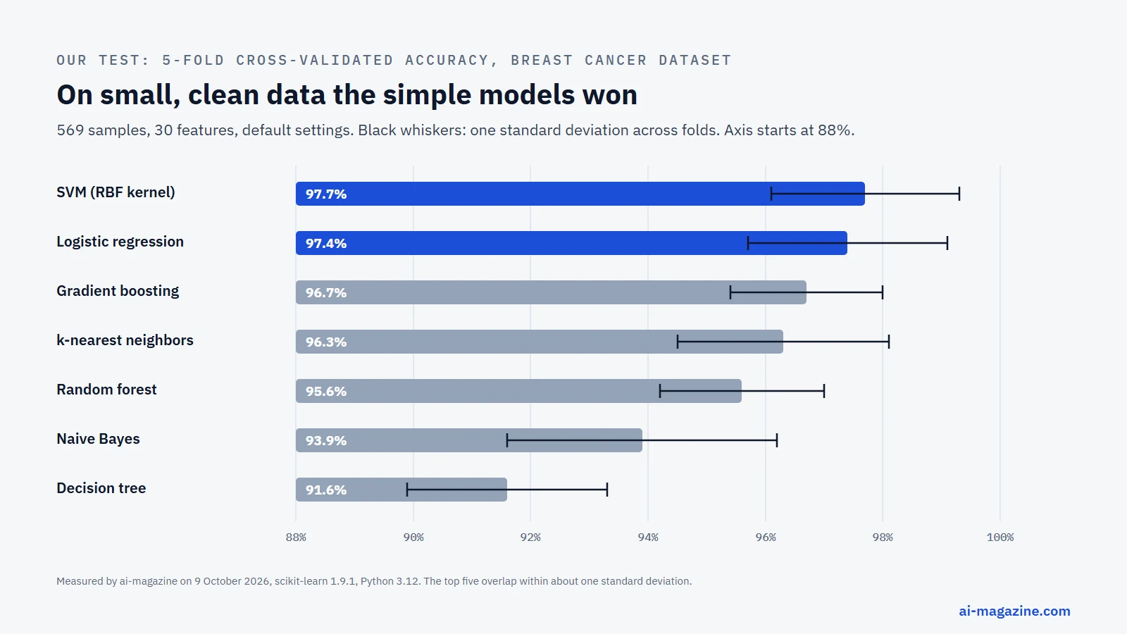
Algorithm	Mean accuracy (5-fold CV)	Std. dev.	Time
SVM (RBF kernel)	97.7%	1.6	0.07 s
Logistic regression	97.4%	1.7	0.35 s
Gradient boosting	96.7%	1.3	1.65 s
k-nearest neighbors	96.3%	1.8	0.18 s
Random forest	95.6%	1.4	3.91 s
Naive Bayes	93.9%	2.3	0.02 s
Decision tree	91.6%	1.7	0.07 s

Three things stand out. First, on a small, clean dataset with well-behaved numeric features, the simple models won: an SVM and plain logistic regression beat both tree ensembles. Second, the top five are within about two percentage points, close to one standard deviation across folds, so the honest conclusion is “several models are equally good here”, not “SVM is best”. Third, a single decision tree trails the forest built from trees by four points, which is exactly the instability that random forests were invented to fix. Run the same script on your own data before trusting any general ranking, including the ones in this article.

A short history of machine learning algorithms

Machine learning has evolved from statistical methods to complex neural networks. The field began with linear regression in 1805, followed by logistic regression in 1958 and the perceptron in 1958. The 1980s brought decision trees and backpropagation, while the 1990s introduced support vector machines and boosting. The 2000s saw the rise of random forests and gradient boosting, dominating tabular data. The 2010s marked the deep learning revolution with AlexNet in 2012 and the transformer in 2017, enabling large language models. Recent years have seen the integration of reinforcement learning, such as RLHF, and the emergence of foundation models for tabular data.

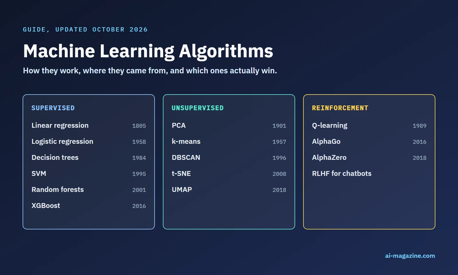
Year	Algorithm	Who
1805	Least squares	Legendre
1901	PCA	Pearson
1951	k-NN	Fix and Hodges
1958	Perceptron	Rosenblatt
1958	Logistic regression	Cox
1957	k-means (Lloyd’s algorithm)	Lloyd, Bell Labs
1967	Name “k-means”	MacQueen
1984	CART	Breiman et al.
1986	Backpropagation	Rumelhart, Hinton, Williams
1986	ID3 decision trees	Quinlan
1989	Q-learning	Watkins
1995	SVM	Cortes and Vapnik
1995	AdaBoost	Freund and Schapire
1996	DBSCAN	Ester et al.
2001	Random Forests	Breiman
2001	Gradient Boosting	Friedman
2008	t-SNE	van der Maaten and Hinton
2012	AlexNet	Krizhevsky, Sutskever, Hinton
2016	XGBoost	Chen and Guestrin
2017	Transformer	Vaswani et al.
2017	LightGBM, CatBoost	Microsoft, Yandex
2018	AlphaZero	Silver et al.
2025	TabPFN	Hollmann et al.

FAQ

What are the main types of machine learning algorithms?

The main types are supervised learning, unsupervised learning, and reinforcement learning. Supervised learning uses labelled data for classification and regression. Unsupervised learning finds hidden structures in unlabelled data, such as clustering or dimensionality reduction. Reinforcement learning learns through trial and error by maximising a reward signal. Semi-supervised and self-supervised learning are also common, using partial or automatically derived labels.

What is the most used machine learning algorithm?

According to the Kaggle 2021 survey, linear or logistic regression is the most used algorithm, cited by 80.3% of data scientists. Decision trees and random forests follow at 74.1%, and gradient boosting machines are used by 59.5%. In the same survey, scikit-learn was used by over 80% of data scientists.

Which machine learning algorithm is best?

There is no single best algorithm; the No Free Lunch theorem formalizes this. The 179-classifier study found random forests the most accurate on average across 121 datasets, and in our own test below an SVM and logistic regression edged out boosting. For tabular data, XGBoost often wins competitions, while deep learning dominates images and text. The best choice depends on your data size, type, and interpretability needs.

What is the difference between supervised and unsupervised learning?

Supervised learning uses labelled data, where the algorithm learns a mapping from inputs to known outputs. It is used for classification and regression. Unsupervised learning uses unlabelled data, finding hidden structures like clusters or reduced dimensions. In supervised learning, you evaluate accuracy against ground truth. In unsupervised learning, you evaluate internal metrics like cluster cohesion or reconstruction error.

Is deep learning better than classic machine learning?

Deep learning is better for unstructured data like images, audio, and text, where it can learn hierarchical features automatically. However, for tabular data, classic machine learning algorithms like XGBoost and random forests often outperform deep neural networks, as shown by Grinsztajn et al. (2022). Deep learning requires more data and compute but can achieve state-of-the-art results in complex perception tasks.

Which algorithm should a beginner learn first?

Begin with linear regression or logistic regression to understand the basics of model fitting and evaluation. Then move to decision trees and random forests, which are intuitive and powerful for tabular data. These algorithms are well-supported by libraries like scikit-learn and provide a solid foundation for understanding bias, variance, and overfitting.

What is the difference between an algorithm and a model?

An algorithm is the procedure or recipe used to learn from data, such as “grow decision trees on bootstrap samples.” A model is the trained result of applying that algorithm, containing the fitted parameters. For example, a decision tree algorithm produces a model that consists of split rules and leaf predictions. The algorithm is the process; the model is the output.

Is XGBoost better than random forest?

XGBoost often outperforms random forest in competitions, as seen in the KDDCup 2015 where it was used by every top-10 team. The XGBoost paper notes that 17 of 29 Kaggle-winning solutions in 2015 used XGBoost. Random forests, though, need far less tuning and are hard to get badly wrong. A sensible approach is to run both with cross-validation; on small datasets the gap is often within noise, as in our test below.

Further reading

• Genetic algorithms explained
• Clustering (glossary)
• A guide to popular AI frameworks: TensorFlow, PyTorch and scikit-learn
• scikit-learn: the machine learning library that isn’t deep learning
• AI algorithms for image recognition
• Free textbooks: The Elements of Statistical Learning (Hastie, Tibshirani, Friedman), An Introduction to Statistical Learning (2021; Python edition 2023), Bishop’s Pattern Recognition and Machine Learning (2006) and Kevin Murphy’s Probabilistic Machine Learning (2022, 2023).