Vector Databases: How They Work and How to Choose One

A vector database stores embeddings, the numeric vectors that represent the meaning of text, images or audio, and finds the ones closest to a query vector. It is the search engine behind retrieval-augmented generation, recommendations, deduplication and image search.

The interesting part is what happens when the collection grows. Comparing a query with every stored vector is exact but slow, so vector databases build indexes that check only a fraction of the data and accept a small chance of missing a true neighbor. This guide explains those indexes, shows measurements from our own machine, covers filtering, quantization, sizing and prices as of September 2026, and ends with how to choose between Postgres and a dedicated database.

What a vector database actually stores

A record in a vector database has three parts:

• An ID that links back to your own data.
• The vector, typically 256 to 3,072 floating-point numbers from an embedding model.
• Metadata, called a payload in Qdrant and metadata in Pinecone: the fields you filter on, such as tenant, language, product or date.

The vector index and the metadata index are separate structures. As Qdrant’s documentation puts it, “a vector index speeds up vector search, and payload indexes speed up filtering”. Pinecone indexes all metadata fields by default and requires flat JSON, with no nesting.

That combination is the job description. A vector database is a store that keeps vectors and their metadata together, searches vectors by distance rather than by equality, and applies metadata filters to that search.

Exact search, and why it stops working

Finding the nearest vectors exactly means computing the distance to every vector in the collection. Qdrant describes the naive approach as one that “would require calculating the distance to every document”. Milvus is equally blunt about the cost of exactness: FLAT “is the only index that can guarantee exact search results”, and it is “the slowest index on our list”.

Exact search is fine more often than people expect. Both Milvus and Faiss recommend it for small collections; Qdrant’s engine switches to a full scan automatically below a configurable threshold, because “using any index would be less efficient than a brute force scan” for roughly the first 10,000 points. Weaviate switches to brute force when a filter is restrictive enough.

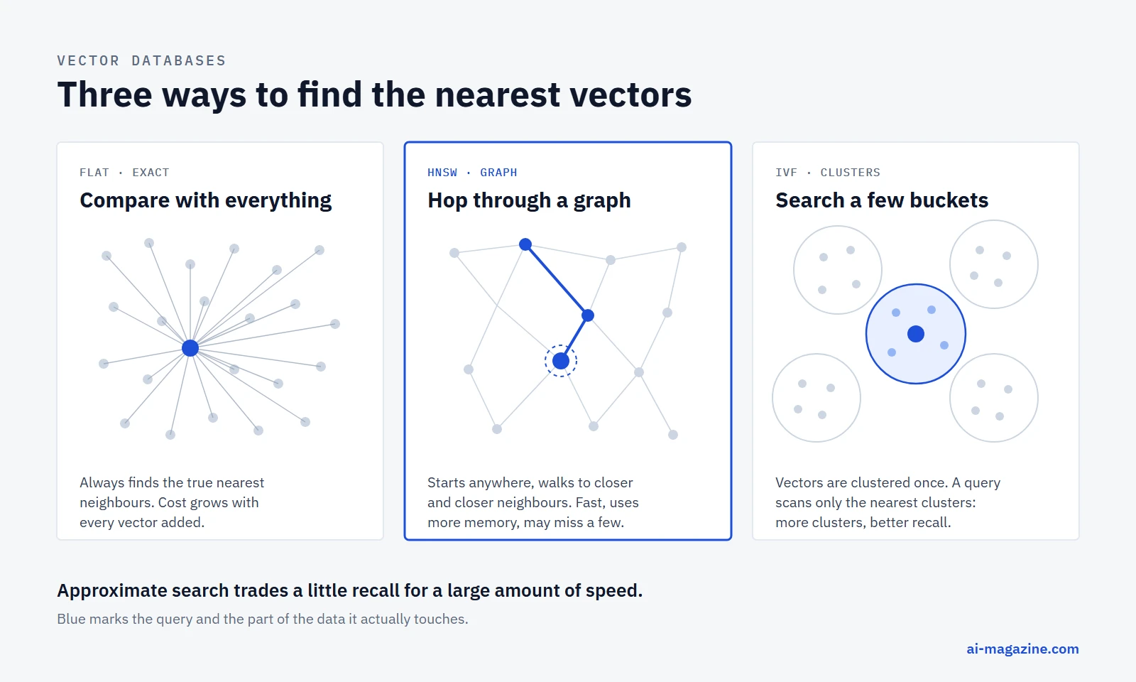
Above that, approximate nearest neighbor (ANN) indexes take over. They come in two main families.

Graph indexes (HNSW) connect each vector to a few of its neighbors and add a hierarchy of long-range links on top. A search starts at an entry point and walks greedily toward the query. The algorithm comes from Malkov and Yashunin’s 2016 paper, which describes layer membership “selected randomly with an exponentially decaying probability distribution” and gives logarithmic scaling.

Clustering indexes (IVF) group vectors into lists around centroids once, then search only the lists nearest to the query. Fewer lists scanned means faster queries and lower recall.

Both are governed by a handful of parameters, and the defaults differ by product:

Product	Max connections per node	Build-time candidate list	Search-time candidate list
pgvector	m = 16	ef_construction = 64	hnsw.ef_search = 40
Qdrant	m = 16	ef_construct = 100	ef = same as ef_construct
Milvus	M = 30	efConstruction = 360	ef = the query’s top-K
Chroma	max_neighbors = 16	ef_construction = 100	ef_search = 100
DuckDB VSS	M = 16	ef_construction = 128	ef_search = 64

Sources: pgvector, Qdrant, Milvus, Chroma, DuckDB. Milvus is inconsistent about its own defaults: its index-selection page lists M = 16 and efConstruction = 200 instead.

The pattern behind the parameters is the same everywhere. A bigger candidate list at build time means a better graph and a slower build; a bigger candidate list at search time means better recall and a slower query. pgvector states it plainly: “A higher value provides better recall at the cost of speed.”

For IVF, pgvector’s guidance is the most concrete published advice: create the index after loading data, use rows / 1000 lists for up to 1M rows and sqrt(rows) above that, and set probes to about sqrt(lists). Its default is one probe, which is why an untuned IVFFlat index returns poor results.

What approximate search buys: our measurement

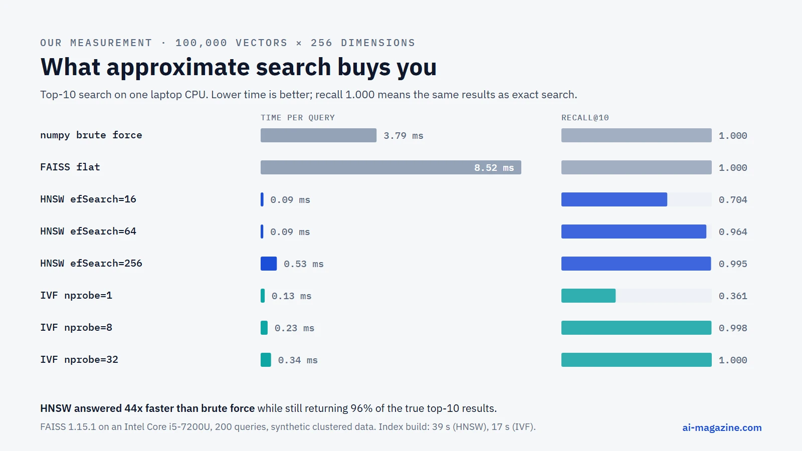
Numbers make the trade-off concrete, so we measured it on an ordinary laptop: 100,000 vectors of 256 dimensions, 200 queries, top-10 results, using FAISS 1.15.1 on an Intel Core i5-7200U. Recall here means the share of the true top-10 that the approximate index returned.

Method	Time per query	Recall@10	Index size
numpy brute force	3.79 ms	1.000	102 MB
FAISS flat (exact)	8.52 ms	1.000	102 MB
HNSW, efSearch 16	0.09 ms	0.704	117 MB
HNSW, efSearch 64	0.09 ms	0.964	117 MB
HNSW, efSearch 256	0.53 ms	0.995	117 MB
IVF, nprobe 1	0.13 ms	0.361	104 MB
IVF, nprobe 8	0.23 ms	0.998	104 MB
IVF, nprobe 32	0.34 ms	1.000	104 MB

Four things stand out, and they generalize even though the exact numbers do not:

• The speedup is large. HNSW answered about 44 times faster than brute force while returning 96% of the true results.
• Recall is a dial, not a property. The same HNSW index went from 0.70 to 0.995 recall by changing one search parameter, and paid for it in time.
• Defaults can be bad. IVF with the default single probe returned barely a third of the right results.
• Indexes cost memory and build time. The HNSW index added 15% on top of the raw vectors and took 39 seconds to build; IVF took 17 seconds.

Two caveats. The data is synthetic and clustered, which flatters IVF: on real embeddings, cluster boundaries are messier. And this is one CPU with 200 queries, not a throughput benchmark. Run the script on your own data before trusting any number, including ours:

import faiss, numpy as np, time

# data: (100_000, 256) float32, L2-normalised; queries: (200, 256)
flat = faiss.IndexFlatIP(256)
flat.add(data)
_, truth = flat.search(queries, 10)          # exact top-10

hnsw = faiss.IndexHNSWFlat(256, 16, faiss.METRIC_INNER_PRODUCT)
hnsw.hnsw.efConstruction = 200
hnsw.add(data)

for ef in (16, 64, 256):
    hnsw.hnsw.efSearch = ef
    t = time.perf_counter()
    _, found = hnsw.search(queries, 10)
    ms = (time.perf_counter() - t) * 1000 / len(queries)
    recall = np.mean([len(set(f) & set(t_)) / 10 for f, t_ in zip(found, truth)])
    print(f"efSearch={ef:3}  {ms:.3f} ms/query  recall {recall:.3f}")

Distance metrics, and the traps in them

Which distance you use has to match the embedding model. Most text embedding models are trained for cosine similarity; some vendors document dot product as equivalent for normalized vectors.

Engine	Cosine	Dot / inner product	Euclidean (L2)	Also supports
Qdrant	yes	yes	yes	Manhattan
Milvus	yes	yes	yes	Hamming, Jaccard (binary)
Weaviate	yes (default)	yes	yes (squared)	Manhattan, Hamming
pgvector	yes	yes	yes	Taxicab, Hamming and Jaccard for bit vectors
Pinecone	yes	yes	yes (squared)	sparse indexes must use dot product
Chroma	yes	yes	yes (default, squared)	—
sqlite-vec	yes	—	yes (default)	L1, Hamming via a function

Three details bite people in production:

• Normalization is sometimes automatic. Qdrant normalizes vectors on upload when the metric is cosine; Weaviate normalizes at read time.
• Some scores are inverted. Weaviate returns the negative dot product so that smaller is always closer. Pinecone’s Euclidean scores are squared distances, where “the most similar results are those with the lowest similarity score”.
• Oracle silently falls back. Query with a different distance function than the index was built with and the index is simply not used.

Filtering: the part that decides your architecture

Most real queries are filtered: this tenant, this language, documents from this year. How a database combines filters with vector search matters more than raw speed.

Post-filtering searches the index first and then drops results that fail the filter. pgvector works this way by default: “With approximate indexes, filtering is applied after the index is scanned.” The failure mode is severe and well documented. With the default hnsw.ef_search of 40, if your filter matches 10% of rows, “only 4 rows will match on average”.

pgvector’s fix, added in 0.8.0, is iterative index scans: the index keeps scanning deeper until enough rows pass the filter. Two modes exist, strict_order and relaxed_order, with caps such as hnsw.max_scan_tuples to bound the work.

Pre-filtering restricts the candidate set before or during the graph traversal. Weaviate builds an allow-list from an inverted index next to the HNSW index and claims that “the recall of a filtered search is typically not any worse than that of an unfiltered search”. Qdrant takes a different route: it extends the HNSW graph with extra edges derived from indexed payload values, with an important operational catch, namely that “extra edges for the HNSW graph can only be generated after payload index creation”. Both now ship ACORN-style strategies for hard filters; in Weaviate, ACORN is the default.

If your product is multi-tenant or filter-heavy, this is the first thing to test, not the last.

Hybrid search and sparse vectors

Dense vectors match meaning; keyword search matches exact terms such as error codes and product names. Most engines now support both in one query:

• Qdrant stores sparse vectors separately, offers a full-text payload index, and fuses rankings with rrf or distribution-based score fusion.
• Milvus supports BM25 as a metric type, sparse indexes, and weighted reciprocal rank fusion, added in 3.0.1.
• Weaviate offers BM25F hybrid search with an alpha weight; since v1.24 its default fusion is relative score fusion rather than RRF.
• Pinecone supports BM25 token matching with Lucene-style syntax and documents RRF as one fusion option.
• pgvector leaves this to Postgres full-text search, with RRF as an example script rather than a built-in.

One trap: the reciprocal rank fusion constant is not universal. Chroma uses the classic k = 60 from the original RRF paper; Qdrant’s default is k = 2 with zero-based ranks. Copying a formula from one product’s docs into another’s setup will change your ranking. Pinecone’s own documentation makes the broader point: “‘Hybrid’ isn’t one fixed method. Qualify what you are combining.”

Quantization: trading precision for memory

A float32 vector of 1,536 dimensions takes about 6 KB. Ten million of them are 61 GB before any index. Quantization shrinks that by storing each number with fewer bits.

Technique	Size reduction	What vendors report
float16 / halfvec	2x	Qdrant: “virtually no impact on the quality of vector search”
Scalar (int8)	4x	Qdrant: error “usually less than 1%”; Milvus IVF_SQ8: 70-75% less memory
Product quantization	up to 64x (Qdrant)	Milvus worked example: 4,096 bits to 512 bits, an 8x reduction
Binary (1 bit)	32x	Qdrant: 0.98 recall@100 on OpenAI 1536-d embeddings with 4x oversampling
Elasticsearch BBQ	32x	“reduces each dimension to a single bit precision”
MongoDB quantization	scalar ~3.75x, binary ~24x in RAM	“the HNSW graph itself does not shrink”

Binary quantization sounds too good until you read the conditions. It works on high-dimensional embeddings with a centered distribution, and it relies on rescoring: the shortlist is re-ranked using full-precision vectors, which must still be stored somewhere. Qdrant enables rescoring by default for binary and its newer TurboQuant encodings.

In pgvector the same idea is a SQL pattern: index binary_quantize(embedding), retrieve a wider candidate set with the Hamming operator, then re-rank the shortlist by exact distance in an outer query. pgvector’s own scaling advice starts with halfvec for “a smaller working set” and moves to binary quantization for “faster build times at scale”.

Sizing: the arithmetic before the shopping

Per-vector storage is simple arithmetic. pgvector documents it exactly: a vector takes 4 * dimensions + 8 bytes, a halfvec takes 2 * dimensions + 8, a bit vector takes dimensions / 8 + 8.

Qdrant publishes the most complete capacity model, including the index:

dense_size = points * dimensions * bytes_per_dimension
hnsw_size  = points * m * 2 * 4 bytes * 1.2
payload    = points * average_payload_size * 1.5

Its own worked example, 1 million points of 768 dimensions with a replication factor of 2:

Component	Size
Raw vectors (float32)	5.72 GB
Same vectors, 4-bit quantized	0.72 GB
HNSW graph	0.29 GB
Payload on disk (1 KB per point)	2.86 GB

Other engines publish comparable formulas: Faiss gives HNSW memory as (d * 4 + M * 2 * 4) bytes per vector, OpenSearch as 1.1 * (4 * dimension + 8 * m), and Weaviate’s own table puts a 1M-vector HNSW index at 2-12 GB depending on dimensions.

Two consequences worth planning for. First, the graph wants to live in RAM: Qdrant notes that graph traversal “does many small random reads that suffer badly from disk latency”. Second, replication multiplies everything, which is why quantization is usually cheaper than another node.

The 2026 landscape

Option	What it is	License	Latest release
pgvector	Vector types and HNSW/IVFFlat indexes inside PostgreSQL	PostgreSQL license	0.8.6, 29 Jul 2026
pgvectorscale	DiskANN-style index and quantization for pgvector, written in Rust	PostgreSQL license	0.9.1, 4 Sep 2026
Qdrant	Vector database with filterable HNSW and tenant-aware storage	Apache 2.0 + cloud	v1.19.1, 4 Sep 2026
Milvus	Distributed vector database, many index types, lake-native in 3.0	Apache 2.0 + Zilliz Cloud	v3.0.1, 9 Sep 2026
Weaviate	Vector database with strong multi-tenancy and pre-filtering	BSD-3-Clause, with parts under the Weaviate License	v1.39.5, 15 Sep 2026
Chroma	Developer-first store: in-process locally, SPANN index in the cloud	Apache 2.0 + cloud	1.5.9, 5 May 2026
Pinecone	Managed, object-storage-native serverless search	Proprietary (also BYOC)	API versioned, e.g. 2026-07
Elasticsearch	Search engine with dense_vector kNN and DiskBBQ	AGPLv3 / SSPL / Elastic License	9.5.4, 15 Sep 2026
OpenSearch	Fork with four pluggable kNN engines, including JVector	Apache 2.0	3.8.0, 5 Aug 2026
Redis	Vector sets data type plus FLAT, HNSW and SVS-VAMANA indexes	RSALv2 / SSPLv1 / AGPLv3	8.10.2, 17 Sep 2026
MongoDB Vector Search	Vector search over documents, managed or self-managed	Server: SSPL; managed in Atlas	Tracks Atlas
sqlite-vec	Brute-force vector search inside SQLite, no server	MIT / Apache 2.0	v0.1.9, 31 Mar 2026
DuckDB VSS	HNSW in DuckDB; persistence still experimental	MIT	Ships with DuckDB
ClickHouse	Vector similarity skip-index, generally available since 25.8	Apache 2.0	LTS 26.8, Sep 2026
LanceDB	Embedded and cloud store on the Lance columnar format	Apache 2.0	0.39.0, 17 Sep 2026
Vespa	Search and ranking engine with vector support	Apache 2.0	8.753.16, 16 Sep 2026

Two notes on licenses, because they changed recently. Weaviate is no longer plain BSD-3: code in its wl/ directory is under a proprietary license gated by a license key. Redis 8 is tri-licensed, with AGPLv3 added rather than substituted.

Also worth knowing: pgvecto.rs is effectively end-of-life and its maintainers point users to VectorChord, which is dual-licensed under AGPLv3 or the Elastic License, so it is source-available rather than clearly open source.

Managed pricing, September 2026

Published list prices, taken from vendor pricing pages on September 18, 2026:

Service	Free tier	Paid model
Pinecone	Starter: 2 GB storage, 2M write units, 1M read units per month	Storage $0.33/GB-month; writes $4-4.50 per million units; reads $16-18 per million units; Standard from $50/month
Zilliz Cloud	5 GB storage, 2.5M vCUs per month, up to 5 collections	Serverless about $4 per million vCUs plus $0.30/GB storage; dedicated from $5-63 per million vectors per month by tier
Weaviate Cloud	100,000 objects, 1 GB memory, 1 cluster	Per million vector dimensions stored: Flex from $0.00465, Premium dedicated from $0.002718; Flex starts at $45/month
Chroma Cloud	$5 credits, 10 databases	Writes $2.50/GiB, storage $0.33/GiB-month, queries $0.0075/TiB scanned
Qdrant Cloud	1 GB RAM, 4 GB disk, free forever	Priced on CPU, memory and disk; no public per-unit rate
OpenAI file search	1 GB storage	$0.10 per GB per day, plus $2.50 per 1,000 tool calls

Pinecone’s units are worth understanding before estimating: a query costs one read unit per gigabyte of namespace scanned, with a 0.25 minimum, which is exactly why Pinecone recommends a namespace per tenant instead of one shared namespace with a tenant filter. Their own example: 100 tenants of 1 GB each cost 1 read unit per query when separated, versus 100 when merged.

Self-hosting shifts the cost to servers and operations. Vendor benchmark claims in this area, such as pgvectorscale’s “28x lower p95 latency” against Pinecone, come from the vendors themselves and have not been independently audited.

Running a vector store with no server at all

Not every project needs a database. For prototypes, desktop apps and test suites, SQLite with the sqlite-vec extension stores vectors in an ordinary file. This script embeds four sentences and answers a question from them:

import sqlite3
import sqlite_vec
from model2vec import StaticModel
from sqlite_vec import serialize_float32

docs = [
    "DeepSeek peak hours are 01:00-04:00 and 06:00-10:00 UTC, Monday to Friday.",
    "Claude Sonnet 5 costs $2 per million input tokens and $10 per million output tokens.",
    "Gemini 3.8 Flash launch pricing ends on December 31, 2026.",
    "A prompt cache hit on Claude Sonnet 5 costs 0.1 times the input price.",
]

model = StaticModel.from_pretrained("minishlab/potion-base-8M")
vectors = model.encode(docs)

db = sqlite3.connect(":memory:")
db.enable_load_extension(True)
sqlite_vec.load(db)
db.enable_load_extension(False)

db.execute("create table documents(id integer primary key, text text)")
db.execute(
    f"create virtual table vec_documents using vec0("
    f"document_id integer primary key, embedding float[{vectors.shape[1]}] distance_metric=cosine)"
)
for i, (text, vec) in enumerate(zip(docs, vectors)):
    db.execute("insert into documents(id, text) values (?, ?)", (i, text))
    db.execute(
        "insert into vec_documents(document_id, embedding) values (?, ?)",
        (i, serialize_float32(vec.tolist())),
    )

query = "how much does caching cost with Claude?"
rows = db.execute(
    """
    select d.text, v.distance
    from vec_documents v
    join documents d on d.id = v.document_id
    where v.embedding match ? and k = 2
    order by v.distance
    """,
    (serialize_float32(model.encode([query])[0].tolist()),),
).fetchall()

for text, distance in rows:
    print(f"{distance:.3f}  {text}")

Its real output on SQLite 3.49.1 with sqlite-vec v0.1.9:

0.509  A prompt cache hit on Claude Sonnet 5 costs 0.1 times the input price.
0.596  Claude Sonnet 5 costs $2 per million input tokens and $10 per million output tokens.

Note the and k = 2 clause: that form works on every SQLite build, while a plain limit requires SQLite 3.41 or newer. Two limits to remember: sqlite-vec is brute-force only, with no ANN index, and its README warns that it “is a pre-v1, so expect breaking changes”.

Operations: what actually goes wrong

Deletes are soft. Every engine marks records as deleted and reclaims space later. Qdrant runs a vacuum optimizer once 20% of a segment is deleted. Milvus is explicit: “storage space will not be immediately released when you delete data”. Weaviate leaves a tombstone until an asynchronous cleanup rebuilds the graph edges, with a default cleanup interval of 300 seconds. In pgvector, “vacuuming can take a while for HNSW indexes”, and the README’s remedy is a concurrent reindex followed by a vacuum. Notably, no vendor publishes a number for how much recall degrades as deletes accumulate, so treat any such claim as unsourced.

Consistency defaults differ. Milvus defaults to bounded staleness. Qdrant defaults to a write consistency factor of 1 and read consistency of 1, and its client libraries disagree on whether writes wait: Python, TypeScript, .NET and Java default to wait=true, Go, Rust and the REST API to false. Weaviate defaults to quorum for both reads and writes. Pinecone is eventually consistent and exposes log sequence numbers so you can tell whether a write is visible yet.

Backups are not all equal. Weaviate supports S3, GCS, Azure and filesystem backends, with incremental backups from v1.37, but restores fail if a collection already exists and do not restore RBAC roles by default. Milvus restores into a new collection, and backups only restore forward within a version line. Pinecone backups are unavailable on the Starter and Builder plans and only include vectors that were in the index at least 15 minutes earlier. With pgvector you use ordinary Postgres tooling, which is a genuine advantage.

Multi-tenancy has documented ceilings. Qdrant Cloud limits a cluster to 1,000 collections by default and recommends payload partitioning or user-defined sharding instead of a collection per tenant. Milvus caps manual partitions at 1,024 per collection and uses a partition key with 16 partitions by default beyond that. Weaviate goes the other way, making a shard per tenant with ACTIVE, INACTIVE and OFFLOADED states, and documents a cluster holding about 170,000 active tenants across nine nodes. Pinecone uses namespaces, capped by plan from 100 to 1,000,000.

Security defaults you should change on day one

• Qdrant’s open-source builds are not secure by default. The documentation is direct: a default deployment “accepts requests from anyone who can reach it”, and internal gRPC traffic “is never protected by an API key nor bearer tokens”, so port 6335 must not be publicly reachable. API keys come in admin, read-only and granular JWT forms.
• Milvus ships a known root password. Authentication is off by default, and when enabled the initial user is root with the password Milvus.
• Weaviate’s RBAC became generally available in v1.29 and must be enabled explicitly; anonymous access is “strongly discouraged except for development or evaluation”.
• Encryption at rest is a cloud feature, not an engine feature. Qdrant Managed Cloud, Pinecone and MongoDB Atlas document encryption at rest; the open-source engines of Milvus and Weaviate do not document it at all, so it falls to your disk or volume encryption.

On top of that, OWASP’s LLM08:2025 Vector and Embedding Weaknesses names the risks specific to this layer: unauthorized access and data leakage through misaligned permissions, cross-tenant context leaks in a shared database, embedding inversion attacks that “recover significant amounts of source information”, data poisoning, and behavior changes caused by retrieved content. Its first mitigation is the one that maps onto everything above: “Ensure strict logical and access partitioning of datasets in the vector database.”

How to choose

Start from the constraints that are hard to change later: where your data already lives, how filtered your queries are, and how many tenants you serve.

Use Postgres with pgvector when your vectors belong next to relational data, your collection is up to a few million vectors, and you value ACID transactions, joins and familiar backups. pgvector’s own pitch is exactly that: “Store your vectors with the rest of your data”, with “ACID compliance, point-in-time recovery, JOINs”. Its documented ceilings are real, though: 2,000 dimensions for an indexed vector column (4,000 with halfvec, 64,000 with binary vectors), post-filtering by default, and slow HNSW vacuuming. pgvectorscale extends the same database with a DiskANN-style index and label-based filtered search.

Use a dedicated vector database when you have tens of millions of vectors or more, heavy filtered search, many tenants, or you need hybrid search and reranking in one query. Qdrant’s filterable HNSW suits filter-heavy workloads; Weaviate’s per-tenant shards suit SaaS products with thousands of isolated datasets; Milvus targets very large distributed deployments and recommends starting with its AUTOINDEX.

Use a managed service when you would rather not operate a stateful system. Pinecone separates storage from compute and bills per read and write unit; Zilliz Cloud and Weaviate Cloud are the managed forms of Milvus and Weaviate; Chroma Cloud suits small teams already using Chroma locally.

Use a library or embedded store when there is no service to operate at all: Faiss inside your own process, sqlite-vec in a file, LanceDB for local multimodal data. Faiss’s guidance is a useful reality check: for a few thousand searches, “just use Flat”, because building an index will not pay for itself. And remember that “all Faiss indexes are stored in RAM”.

If you already run Elasticsearch, OpenSearch, Redis, MongoDB or ClickHouse, check their vector support before adding a system. All five now index vectors, and one fewer moving part is usually worth more than a benchmark win.

Benchmark claims, and how to test properly

Every vendor publishes numbers that favour it. Milvus claims “2-5x” better performance than other vector databases; pgvectorscale claims large wins over Pinecone; turbopuffer publishes both fast and slow figures. None of these are independently audited.

The long-standing neutral benchmark, ann-benchmarks.com, measures recall against queries per second on standard datasets under a single-CPU constraint. It is also, in its maintainers’ own words, “no longer actively maintained”, with published results frozen at April 2025 and a pointer to a successor, VIBE. Even VIBE scopes itself carefully: “we do not aim to benchmark vector databases or cloud services”. It compares algorithms, not products.

So the only benchmark that settles your decision is your own:

1. Take 10,000 or more of your real embeddings and 50 to 100 real queries.
2. Compute exact top-10 results once with brute force. That is your ground truth.
3. Measure recall and latency for each candidate at several settings of its search parameter.
4. Repeat with your real filters applied; this is where products differ most.
5. Include index build time and memory, then check the cost of that memory at your target scale.

Frequently asked questions

Do I need a vector database for RAG?

Not always. For a few thousand chunks, vectors in memory, in SQLite or in a Postgres table are enough. A dedicated database earns its place with large collections, filtered queries, many tenants, or built-in hybrid search.

Is pgvector fast enough for production?

For millions of vectors on a well-sized instance, yes, and plenty of products run on it. Watch three things: indexed dimensions are capped at 2,000 for the vector type, filtering is post-filtering unless you enable iterative scans, and HNSW index maintenance is slow enough to plan around.

What is the difference between HNSW and IVF?

HNSW builds a navigable graph and searches by hopping toward the query: fast and accurate, with higher memory use and slower builds. IVF clusters vectors and scans only the nearest clusters: cheaper to build and smaller, with recall that depends heavily on how many clusters you probe.

How much recall do I lose with approximate search?

You choose. In our test, HNSW returned 96% of exact results at default-like settings and 99.5% with a larger candidate list, at five times the latency. Measure it on your data: recall depends on the index parameters, the data distribution and your filters.

Can I use a normal database instead?

Increasingly yes. PostgreSQL, MySQL HeatWave, Oracle, MongoDB, Redis, ClickHouse, Elasticsearch and SQLite all have vector support now. The questions to ask are which index types they offer, whether filters are applied before or after the vector search, and what happens to recall at your scale.

What happens when embeddings change?

Changing the embedding model means re-embedding and re-indexing everything, because vectors from different models are not comparable. Plan for re-indexing as a routine operation: keep the source text, store the model name and version with each vector, and make the pipeline repeatable.

Related

• What is RAG?, the main application of vector search
• Vector database, embedding and semantic search in the glossary
• LLM API pricing and the LLM API cost calculator for the generation side of the bill