Machine Learning vs Deep Learning: The Real Differences and When to Use Each (2026)

Deep learning is a subset of machine learning that uses many-layered neural networks to learn its own features from raw data. Classical machine learning works best on tables of numbers and small data, while deep learning dominates when you are dealing with images, text, audio, or massive datasets. That is the short answer. In 1959, Arthur Samuel already weighed a “neural-net approach” against a “much more efficient”, highly organized one in his checkers paper, so the debate is older than most of today’s software. We also ran our own test on clothing photos and house-price data to check the most repeated rule of thumb, that deep learning only wins with lots of data; the type of data turned out to matter more than the amount. This guide breaks down exactly how these technologies differ in structure, data requirements, and real-world application.

Machine learning vs deep learning at a glance

	Classical machine learning	Deep learning
What it is	Algorithms that learn patterns from data	Machine learning with many-layered neural networks
Features	Mostly chosen and prepared by people	Learned from raw data by the network
Best data	Tables of numbers and categories	Images, audio, video, text
Data needed	Works from hundreds to thousands of rows	Best results with very large datasets or a pretrained model
Hardware	An ordinary CPU, often seconds to minutes	GPUs or TPUs, from hours to months for the largest models
Explaining decisions	Often readable (trees, coefficients)	Needs separate tools such as SHAP
Typical algorithms	Linear and logistic regression, decision trees, random forests, gradient boosting, SVM, k-means	CNNs, RNNs and LSTMs, transformers, diffusion models
Everyday examples	Credit scoring, fraud rules, sales forecasts	Photo search, speech recognition, ChatGPT

AI vs machine learning vs deep learning

To understand the difference between machine learning and deep learning, you first need to see how they fit into the broader field of artificial intelligence. The relationship is hierarchical. Artificial intelligence is the broadest category, encompassing any system that mimics human intelligence. Machine learning is a subset of AI: in the book’s words, systems that acquire their own knowledge “by extracting patterns from raw data”. Deep learning is a further subset of machine learning that uses neural networks with many layers to learn representations of data.

The Deep Learning textbook by Goodfellow, Bengio, and Courville visualizes this clearly. AI includes everything from knowledge bases to search algorithms. Machine learning includes techniques like logistic regression, which in the book’s example decides whether to recommend a cesarean delivery based on patient data. Representation learning, which sits between machine learning and deep learning, involves using machine learning to discover not just the mapping from data to output, but also the representation itself. Deep learning, specifically deep neural networks like multi-layer perceptrons (MLPs), solves this representation problem by introducing layers that express complex concepts in terms of simpler ones.

The term “deep learning” has a surprisingly long history. It was used as early as 1986 in the context of constraint-satisfaction problems and in 2000 in relation to multi-valued neurons. However, it was popularized after 2006, when researchers like Geoffrey Hinton demonstrated that deep networks could be trained effectively.

Arthur Samuel, who popularized the phrase machine learning, described his 1959 work as programming a computer “to behave in a way which, if done by human beings or animals, would be described as involving the process of learning”, and predicted that “programming computers to learn from experience should eventually eliminate the need for much of this detailed programming effort.” The definition most textbooks use today comes from Tom Mitchell’s 1997 book: “A computer program is said to learn from experience E with respect to some class of tasks T and performance measure P, if its performance at tasks in T, as measured by P, improves with experience E.” In practice, this means a machine learning model improves at a task, like classifying emails as spam, as it processes more labeled examples.

A neural network is a computational model inspired by the biological brain. It consists of layers of interconnected nodes or “neurons.” Every network has an input layer and an output layer; the layers in between are called hidden layers. There is no official cutoff for “deep”, but a network with more than one hidden layer is usually called a deep neural network, and modern image and language models have dozens or hundreds of layers. This depth allows the network to learn hierarchical features. The first layers might learn simple edges in an image, while deeper layers learn complex shapes or objects. This is the core of the difference between deep learning and neural networks: all deep learning uses neural networks, but not all neural networks are deep. Shallow networks with one hidden layer are often sufficient for simpler problems, but deep networks are required for the complexity of modern data like language and video.

How they work differently

Features: engineered by people vs learned from data

The most practical difference lies in how features are handled. In classical machine learning, you must manually engineer features. If you are predicting house prices, you need to provide the algorithm with specific columns: square footage, number of bedrooms, zip code, and age of the house. The algorithm learns the relationship between these predefined columns and the price. You need domain expertise to decide which columns matter. If you miss a crucial feature, like the proximity to a good school, the model’s performance will suffer because it doesn’t know to look for it. This work is called feature engineering.

Deep learning automates this feature extraction. Instead of providing labeled columns, you feed the raw data into the network. If you are recognizing a cat in an image, you don’t tell the network what a cat looks like. You feed it millions of images, and the network automatically learns which pixels and patterns constitute a cat. The early layers of the network learn low-level features like edges and textures. Deeper layers combine these to recognize shapes, and the final layers recognize the complete object. This ability to learn features directly from raw data is why deep learning excels at unstructured data like images, audio, and text.

Data: how much each needs

Classical machine learning models are highly efficient with small to medium datasets. A random forest or gradient boosting machine can often achieve excellent results with just a few thousand rows of data. These models are robust and do not require massive amounts of information to converge. In fact, on typical tabular data, tree-based models often outperform deep learning because they can capture complex interactions without needing huge volumes of examples.

Deep learning is data-hungry. It thrives on massive datasets. Google researchers who trained on 300 million images found that accuracy on vision tasks grows roughly with the logarithm of the data: more data keeps helping, with diminishing returns. Without enough data, deep networks tend to overfit, meaning they memorize the training data rather than learning generalizable patterns. This is why deep learning became feasible only recently. The availability of big data and the computational power to process it have been the primary drivers of the deep learning revolution. If you have a small table of numbers, classical machine learning is usually the safer choice. Small sets of images or text are a different story, as our test below shows, especially when you can start from a pretrained model (transfer learning).

Hardware and training time

The hardware requirements for these two approaches differ significantly. Classical machine learning models can be trained on a standard CPU in seconds or minutes. A gradient boosting model on a dataset of 10,000 rows might take less than a minute to train on a laptop. This speed makes them ideal for rapid prototyping and environments where compute resources are limited.

Deep learning typically requires specialized hardware, such as Graphics Processing Units (GPUs) or Tensor Processing Units (TPUs). These devices are designed to handle the massive matrix multiplications involved in neural network training. Training a deep neural network can take hours, days, or even weeks, depending on the model size and dataset. Energy use is far higher too: we come back to the numbers in the cost section below. This hardware dependency adds to the cost and complexity of deploying deep learning solutions at scale.

Interpretability

Explainability is a critical factor in regulated industries like finance and healthcare. Classical machine learning models are generally more interpretable. A decision tree can be visualized as a flowchart, making it easy to see exactly why a specific decision was made. A linear regression model provides coefficients that indicate the impact of each feature on the outcome. You can explain to a customer why their loan was denied by pointing to specific variables.

Deep learning models are often referred to as “black boxes.” While they are incredibly accurate, understanding why they make a specific decision is difficult. A neural network with millions of parameters does not have a simple visual representation. Researchers use explainable AI tools like SHAP (SHapley Additive exPlanations) to assign importance values to features, but these are approximations. The model itself does not provide a clear, logical path from input to output. This lack of transparency can be a barrier in contexts where regulatory bodies require detailed explanations for automated decisions.

Typical algorithms on each side

Classical machine learning relies on algorithms that are well-understood and mathematically grounded. These include linear and logistic regression, decision trees, random forests, gradient boosting machines (like XGBoost and LightGBM), support vector machines (SVM), and k-means clustering. They usually need less tuning and perform very well on structured data. Our guide to machine learning algorithms explains each one with a diagram.

Deep learning utilizes neural network architectures designed for specific types of data. Convolutional neural networks (CNNs) are the standard for image recognition. Recurrent Neural Networks (RNNs) and Long Short-Term Memory (LSTM) networks are used for sequence data like time series or text. Transformers, which rely on attention mechanisms, have revolutionized natural language processing and are now used in various domains. Diffusion models are leading the field in image generation. Each architecture is optimized for the specific structure of the data it processes.

A short history, from checkers to Nobel Prizes

The journey from checkers to Nobel Prizes illustrates the evolution of these technologies. In 1959, Arthur Samuel published “Some Studies in Machine Learning Using the Game of Checkers” in the IBM Journal of Research and Development. In this paper, he described a program that learned to play checkers better than its creator. Samuel contrasted a “neural-net approach”, a randomly connected network trained by reward and punishment, with a highly organized approach built around features he chose himself, and judged the organized one “much more efficient”. His program learned to beat its author after 8 to 10 hours of playing time. His work demonstrated that computers could learn from experience, a core principle of machine learning.

The field experienced three distinct waves. The first wave, cybernetics, ran from the 1940s to the 1960s, focusing on control systems and early neural models. The second wave, connectionism, spanned from 1980 to 1995. This era saw the popularization of backpropagation, a method for training neural networks, notably through the work of Rumelhart, Hinton, and Williams in 1986. However, the field faced challenges with training deep networks, leading to a period of reduced interest.

The third wave, deep learning, began around 2006. Geoffrey Hinton and his colleagues published papers on deep belief networks, demonstrating that layer-wise pre-training could effectively initialize deep networks. Training one layer at a time made it practical to train networks with many layers, and the term “deep learning” was popularized in this period, though it had been used earlier.

The field accelerated rapidly with AlexNet in 2012. This convolutional neural network, trained on the ImageNet dataset, achieved a top-5 error rate of 15.3% in the 2012 ImageNet challenge, against 26.2% for the second-best entry. It used GPUs for training and demonstrated the power of deep learning on large-scale data. This event marked a turning point, convincing many researchers that deep learning was the future of computer vision.

In 2017, the Transformer architecture was introduced in the paper “Attention Is All You Need.” It dispensed with recurrence and convolutions entirely, relying solely on attention mechanisms. This architecture became the foundation for large language models (LLMs) and transformed natural language processing.

The recognition of these achievements culminated in major awards. In 2018, Yoshua Bengio, Geoffrey Hinton, and Yann LeCun received the ACM A.M. Turing Award for their conceptual and engineering breakthroughs that made deep neural networks a critical component of computing. In 2024, Geoffrey Hinton and John Hopfield were awarded the Nobel Prize in Physics for foundational discoveries that enable machine learning with artificial neural networks. That same year, half of the Nobel Prize in Chemistry went to Demis Hassabis and John Jumper of Google DeepMind for protein structure prediction with AlphaFold2, a deep learning system that predicted the structure of virtually all 200 million proteins researchers have identified; the other half went to David Baker for computational protein design. These awards signal that machine learning and deep learning are no longer just computer science topics but fundamental scientific advances with profound implications for biology, physics, and beyond.

When classical machine learning wins

The narrative that deep learning has rendered traditional algorithms obsolete often ignores the reality of everyday business data. For structured, tabular information—rows and columns of numbers, dates, and categories—gradient-boosted decision trees remain the gold standard. A comprehensive analysis by Grinsztajn, Oyallon, and Varoquaux published at NeurIPS 2022 examined 45 datasets with approximately 10,000 samples and found that tree-based models consistently outperform deep learning on medium-sized data, even without accounting for their superior speed. The study identified that neural networks struggle to be robust to uninformative features, preserve the orientation of the data, and learn irregular functions without significant effort.

The debate is further nuanced by Shwartz-Ziv and Armon, whose 2022 research demonstrated that XGBoost beats deep models across various datasets, including those specifically designed to favor neural networks. Crucially, XGBoost requires significantly less hyperparameter tuning to reach that performance level. They also noted that an ensemble combining deep models with XGBoost often beats XGBoost alone, suggesting that hybrid approaches are already the pragmatic choice. Similarly, McElfresh et al. analyzed 176 datasets in 2023 and concluded that the “neural network vs. boosted tree” debate is overemphasized. For many datasets, the performance difference is negligible, and light hyperparameter tuning on a Gradient Boosted Decision Tree (GBDT) matters more than the fundamental choice between NNs and GBDTs. GBDTs are particularly better suited for handling skewed or heavy-tailed feature distributions common in business data.

An older and broader benchmark points the same way: Fernández-Delgado and colleagues compared 179 classifiers on 121 datasets in 2014, and random forests came out best, reaching 94.1% of the maximum accuracy on average. Industry adoption reflects this. The Bank of England and the FCA reported in 2024 that gradient boosting comprises 32% of all reported AI use cases in UK financial services, far outpacing other model types. In machine learning competitions, the dominance of trees is undeniable. The 2024 State of ML Competitions report noted that among 400+ competitions, PyTorch and gradient-boosted tree models were the most common tools among winners; 16 winning solutions used LightGBM, 13 CatBoost and 8 XGBoost, and tree models still dominated tabular and time-series problems. No single deep-learning architecture has emerged to dominate these specific problem types.

Even tech giants have relied on this logic. Uber’s ETA prediction system originally used a group of XGBoost models, each trained on a specific mega-region, because XGBoost was widely considered the best-in-class for modeling tabular data. Stripe’s Radar fraud detection system used a “Wide & Deep” ensemble of XGBoost and neural networks until 2022. Stripe noted that while XGBoost is not a cutting-edge technique, it provided unique value, and removing it naively would have cost them 1.5% recall. For most businesses dealing with structured data, starting with a strong gradient boosting baseline is not just a fallback—it is often the optimal choice.

When deep learning wins

Deep learning truly shines when the data is unstructured or when scale is the primary driver of performance. This includes images, speech, text, and video. The field’s turning point arrived with AlexNet in 2012, which achieved a top-5 test error rate of 15.3% on the ImageNet Large Visual Recognition Challenge, compared to 26.2% for the second-best entry. Trained on GPUs with 60 million parameters, AlexNet demonstrated that deep convolutional neural networks could extract features from raw pixels better than hand-engineered methods.

The power of deep learning is fundamentally tied to data volume and compute. Research by Sun et al. in 2017 analyzed 300 million images and found that performance on vision tasks increases logarithmically based on the volume of training data. Hestness et al. confirmed this with a power-law generalization error scaling across four domains, showing that model improvements shift error but do not affect the underlying scaling exponent. Kaplan et al. formalized this with “scaling laws,” showing that loss scales as a power-law with model size, dataset size, and compute. This means that larger models are more sample-efficient, provided you have the data to feed them.

DeepMind’s 2022 Chinchilla study refined this: for every doubling of model size, the number of training tokens should also be doubled. Chinchilla, with 70 billion parameters, used the same compute as the 280-billion-parameter Gopher but four times more data, and beat both Gopher and the 175-billion-parameter GPT-3. Andrew Ng’s famous data-vs-performance curve illustrates this dynamic: traditional algorithms like logistic regression plateau once they have seen enough data, while neural networks continue to improve as data scales. However, Ng includes a crucial caveat: in the regime of small training sets, the relative ordering of algorithms is not well-defined, and performance depends heavily on feature engineering skills. Only in the “very large” regime do large neural networks consistently dominate.

This scale advantage enables breakthroughs in fields previously dominated by human expertise. AlphaFold2, developed by Google DeepMind, predicted the structure of virtually all 200 million identified proteins, a feat that earned Demis Hassabis and John Jumper the 2024 Nobel Prize in Chemistry. Similarly, the Transformer architecture, introduced in 2017, dispensed with recurrence and convolutions entirely, relying solely on attention mechanisms. This architecture became the foundation for Large Language Models (LLMs), which now power everything from search engines to code assistants. When the data is unstructured, high-dimensional or vast, deep learning is the approach that keeps improving with scale.

Our test: does deep learning really need more data?

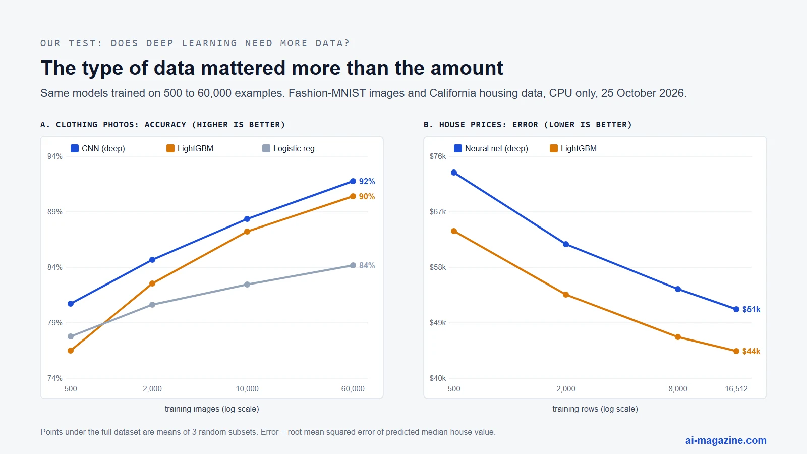
The most repeated rule of thumb is that classical machine learning wins on small data and deep learning only pulls ahead with lots of it. Andrew Ng’s well-known curve says roughly that, though he adds that with small training sets the ranking is “not very well defined”. We tested it on 25 October 2026 on an ordinary CPU, training the same models on growing slices of two standard datasets and scoring them on the same held-out test data each time:

• Images: Fashion-MNIST, small grayscale photos of clothing in 10 classes, with 500, 2,000, 10,000 and all 60,000 training images. Classical models: logistic regression and LightGBM (gradient-boosted trees) on raw pixels. Deep model: a small convolutional neural network (CNN) in PyTorch.
• A table: California housing, 8 numeric columns per district, with 500, 2,000, 8,000 and all 16,512 training rows. Classical model: LightGBM. Deep model: a two-layer neural network (MLP).

Each point below the full dataset is the average of three random subsets.

Training examples	Images: CNN	Images: LightGBM	Images: logistic regression	Table: LightGBM error	Table: neural net error
500	80.8%	76.5%	77.8%	$63,900	$73,400
2,000	84.7%	82.6%	80.6%	$53,600	$61,700
8,000 to 10,000	88.4%	87.2%	82.5%	$46,700	$54,500
Full set (60,000 / 16,512)	91.8%	90.4%	84.2%	$44,400	$51,200

On images, the deep model led at every size, including the smallest. With only 500 training photos the CNN reached 80.8%, ahead of both classical models. A convolutional network is built to look for edges and shapes in neighboring pixels, and that built-in assumption helps even when examples are scarce. Gradient boosting started last at 500 images but improved fastest, closing to within 1.4 points at 60,000.

On the table, gradient boosting led at every size, including the largest. LightGBM’s error was about 13-14% lower than the neural network’s across the whole range, and adding data did not close the gap: both improved at a similar pace.

What this means: in our test the type of data predicted the winner better than the amount. “Deep learning needs big data” is true in the sense that its best results come at huge scale, and that very large models need far more data than we used here. But the decision you face first is usually simpler: neural networks for images, sound and text, gradient-boosted trees for tables of numbers, then check on your own data.

Limits: two small public datasets, one run of each configuration per subset, no tuning, CPU only. Logistic regression is shown for images only. A pretrained network fine-tuned on our 500 photos would likely have done even better, which is how deep learning is usually applied to small datasets today.

The line is blurring: deep learning for tables

The boundary between classical machine learning and deep learning is becoming increasingly porous. Researchers are now applying deep learning architectures to tabular data, often with surprising results. A January 2025 paper in Nature introduced TabPFN, a tabular foundation model that beats a four-hour tuned ensemble of gradient-boosted trees in just 2.8 seconds on datasets up to 10,000 samples. TabPFN uses a transformer trained on millions of synthetic datasets to make accurate predictions on small data, challenging the 20-year dominance of gradient-boosted decision trees.

TabPFN-2.5, described in the developer Prior Labs’ own technical report in November 2025 (not yet independently replicated), extends this capability to 50,000 rows and 2,000 features, a 20-fold increase in data cells. It matches the performance of AutoGluon, a four-hour tuned ensemble, and achieves a 100% win rate against default XGBoost on small-to-medium classification tasks. The model can be distilled into an MLP or tree ensemble for low-latency production use, bridging the gap between high-accuracy research models and practical deployment.

This blurring is also evident in hybrid approaches. Shwartz-Ziv’s work showed that ensembling deep models with XGBoost often yields superior results. Stripe’s evolution from an XGBoost+DNN ensemble to a DNN-only architecture in 2022 further illustrates this shift. By removing the XGBoost component, Stripe cut training time by over 85% to less than two hours, proving that deep learning can handle tabular fraud detection efficiently at scale. These developments suggest that the choice is no longer strictly between “trees” and “neural networks,” but rather about selecting the right architecture for the specific data scale and latency requirements.

Cost, compute and energy

The resource requirements for deep learning are substantial and growing. Training compute for notable AI models has grown by approximately 4.1x per year between 2010 and May 2024, with frontier models growing at a 4–5x annual rate. The amortized hardware and energy cost of final training runs has grown 2.4x per year since 2016. Based on current trends, the largest training runs are expected to exceed $1 billion by 2027.

Energy consumption is a major component of this cost. Global data centers consumed 415 TWh of electricity in 2024, accounting for 1.5% of world electricity, according to the IEA. This is projected to rise to 945 TWh by 2030, slightly more than Japan’s total current electricity consumption. AI is the most important driver of this growth. Within machine learning workloads, inference represents about three-fifths of total energy usage at Google, so at Google, running models used more energy than training them.

The financial scale of frontier training is already staggering. Estimates place the training cost of GPT-4 at approximately $78 million and Gemini Ultra at $191 million. Grok 4 by xAI, the largest training run Epoch AI had analyzed as of September 2025, is estimated to have consumed 310 GWh of electricity and cost around $490 million in compute. Epoch stresses that these numbers are uncertain, based on vague public statements, but they are indicative of the scale required for state-of-the-art deep learning.

Despite these costs, inference prices are dropping rapidly. The Stanford AI Index reports that GPT-3.5-level inference cost fell from $20.00 to $0.07 per million tokens between November 2022 and October 2024, a more than 280-fold decrease. This makes deep learning accessible for many applications, even if the initial training remains expensive. For most businesses, however, classical machine learning remains significantly cheaper to train and deploy, often on a laptop CPU, while deep learning requires specialized hardware and significant energy budgets.

Explainability and regulation

As AI systems make more critical decisions, the need for explainability has moved from academic interest to regulatory requirement. The EU GDPR Articles 13-15 and 22 mandate that data subjects have the right to “meaningful information about the logic involved” in automated decisions that produce legal effects. The EU AI Act (Annex III, point 5(b)) designates AI systems used for credit scoring as high-risk, and Article 86 gives affected persons the right to obtain clear and meaningful explanations of the AI system’s role in the decision-making procedure.

In the United States, the CFPB Circular 2022-03 clarified that creditors using complex algorithms must still provide specific principal reasons for adverse action. The notice rules apply equally to all credit decisions, regardless of the technology used. Crucially, the Circular states that a creditor’s “lack of understanding of its own methods is therefore not a cognizable defense.” This means that using a black-box deep learning model does not excuse a bank from explaining why it denied a loan.

To address this, researchers developed SHAP (SHapley Additive exPlanations) in 2017, a method that assigns each feature an importance value per prediction, unifying six existing interpretability methods. This is one reason gradient boosting, the most common model type in UK financial services, is often paired with explanation tools or simple scorecards rather than replaced by deep networks. FICO, for example, describes on its blog a “Teacher–Student” approach, where a complex ML teacher model is distilled into a segmented scorecard that is almost as predictive but easier to explain. This hybrid approach allows financial institutions to maintain high accuracy while satisfying regulatory demands for transparency.

How to choose between machine learning and deep learning

Choosing between machine learning and deep learning is not about picking the most advanced technology, but the most appropriate one for your specific constraints. Follow this checklist to decide:

1. Data type: Is your data structured (tabular) or unstructured (images, text, audio)? Use gradient boosting for tabular data; use deep learning for unstructured data.
2. Amount of labelled data: Do you have thousands or millions of examples? Deep learning thrives on large datasets; classical ML often performs better or equal on small-to-medium datasets.
3. Need to explain decisions: Do regulators or stakeholders require you to explain why a decision was made? If yes, start with gradient boosting or logistic regression, which are more interpretable, or use SHAP values to explain deep models.
4. Hardware and budget: Do you have access to GPUs and a large energy budget? Classical ML can often be trained on a laptop CPU; deep learning usually requires specialized hardware.
5. Latency: Do you need real-time inference with low latency? Small tree ensembles and linear models are cheap to run on ordinary servers; large neural networks may need GPUs to answer quickly, though they can be distilled into smaller models.
6. Existing pretrained models: Can you use transfer learning or LLM APIs? If yes, deep learning offers a shortcut to high performance without training from scratch, even with only a few hundred labelled examples.
7. Start with a strong baseline: Always begin with a gradient boosting model. Only move to deep learning if it clearly wins on a held-out test set, justifying the added complexity and cost.

Frequently asked questions

What is the main difference between machine learning and deep learning? Machine learning is the broader field of algorithms that learn from data, while deep learning is a subset of ML that uses multi-layered neural networks. Deep learning automatically learns hierarchical features from raw data, whereas traditional ML often requires manual feature engineering.

Is deep learning better than machine learning? Not universally. Deep learning excels with unstructured data like images and text, especially at scale. However, for structured tabular data, classical machine learning models like gradient boosting often outperform deep learning with less data and compute.

Is deep learning a subset of machine learning? Yes. Deep learning is a kind of representation learning, which is in turn a kind of machine learning. It achieves power by representing the world as a nested hierarchy of concepts, with each concept defined in relation to simpler ones.

What is the difference between AI, machine learning and deep learning? Artificial Intelligence is the broadest term, covering any system that mimics human intelligence. Machine Learning is a subset of AI that uses algorithms to learn patterns from data. Deep Learning is a subset of ML that uses neural networks with many layers.

Is a neural network deep learning? Not necessarily. A neural network with a single hidden layer is usually called shallow. Deep learning specifically refers to neural networks with many layers (deep architectures) that can learn complex, hierarchical representations.

Does deep learning always need big data? No. Its best results come at very large scale, but in our test a small convolutional network trained on just 500 clothing photos already beat logistic regression and gradient boosting. On tables of numbers, gradient boosting won at every size we tried, so the type of data matters more than the amount.

Which should I learn first? Start with classical machine learning. It is easier to understand, requires less compute, and is highly effective for many real-world problems. Once you grasp the fundamentals, move to deep learning to handle unstructured data and large-scale challenges. Our guide to TensorFlow, PyTorch and scikit-learn shows which library fits each step.

Is ChatGPT machine learning or deep learning? ChatGPT is deep learning. It is built on the Transformer architecture, a type of deep neural network, and uses large language models trained on vast amounts of text data to generate human-like responses.